The first model I trained on this data had an AUC of 0.96. For origination-only small-business credit, that is not a good result. It is a warning.
This note walks through an end-to-end credit model built on 772,591 real US Small Business Administration loans, from raw government data to a default model, a loss model, expected loss, risk-based pricing and an approval policy. Every number below is reproducible from the public code. The most useful finding is the 0.96 I didn't keep.
Executive summary
The question. Can origination data alone rank small-business borrowers well enough to set approvals and prices, and does that ranking survive a downturn?
The approach. Take every resolved SBA loan from 1990 to 2007, build features the way a lender could have known them at approval, train on the 1990s and early 2000s, and test on the 2006–07 loans that defaulted at five times the normal rate in the crisis.
The answer. A constrained gradient-boosted model ranks borrowers better than a traditional scorecard in every year tested (AUC 0.664 versus 0.616), and at the same approval rate it swaps 45%-bad loans for 31%-bad loans. Origination data caps performance near 0.66, and the default level needs a separate stress adjustment in a downturn.
The decision it supports. Use the constrained model as champion with the scorecard as challenger, price from its risk deciles, set cutoffs on profit, treat leakage testing as mandatory, and add cash-flow data to break through the ceiling.
Business outcomes
What the model changes for a lender, on the 2006–07 crisis cohort it never saw in training:
| Business lever | Scorecard today | With the new model | What it means |
|---|---|---|---|
| Who gets approved | Approves a set with a 45% bad rate that the new model would decline | Swaps in a set with a 31% bad rate | Same approval rate, same volume, better borrowers |
| Defaults at the same volume | Baseline | About 2,000 fewer defaulted loans across the 14,687 swapped | Fewer charge-offs without shrinking the book |
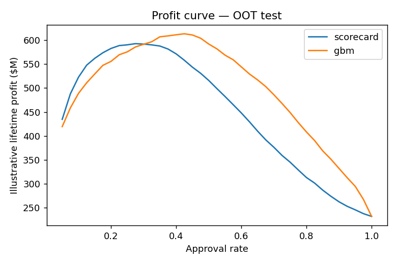
| Portfolio profit | Baseline at its best cutoff | +$21M illustrative lifetime profit at its best cutoff | The ranking gain turns into money once cutoffs are set on profit |
| Pricing | One rate band for most borrowers | Indicated rate from about 8.8% to 13.6% by risk decile | Price follows risk instead of averaging it |
| Reserve and capital planning | Predicted 26% default against 39% actual in the downturn | Stress overlay cuts calibration error from 0.128 to 0.077 | Loss forecasts that hold up when the cycle turns |
| Model risk | A 0.96 AUC that would have failed in production | Leakage caught and the field removed before use | No false confidence reaching the credit committee |
| Early warning | Drift found after losses arrive | Population stability index of 1.64 flags the shift for review | Retrain triggered by data, not by losses |
Defaults avoided are derived from the swap-set: 14,687 × (45% − 31%). Profit uses illustrative pricing, not any lender's economics.
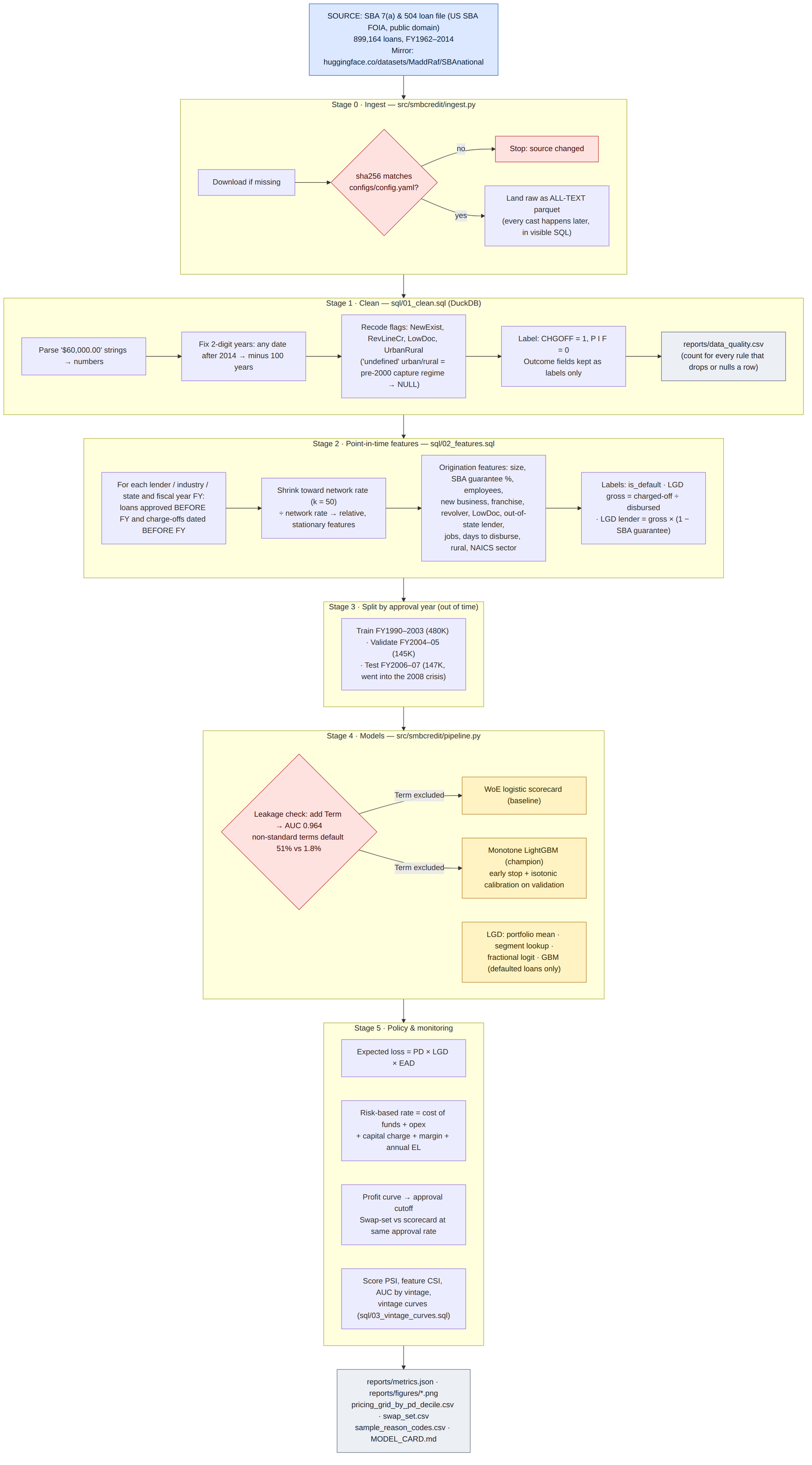
End to end in six steps
| Step | What happens | Output |
|---|---|---|
| 1. Source | Download the SBA 7(a) and 504 loan file (FOIA, public domain) and verify its checksum | 899,164 raw loans |
| 2. Clean | Type every field in SQL, fix two-digit years and coded flags, count every rule that drops or changes a row | Clean loan table and a data-quality report |
| 3. Engineer features | Origination fields plus lender, industry and state loss history, using only outcomes known before each loan | 17 features per loan |
| 4. Split by time | Train FY1990–2003, validate FY2004–05, test FY2006–07 | 480K / 145K / 147K loans |
| 5. Model | Leakage check, scorecard versus constrained gradient-boosted model, calibration, loss-severity model | Probability of default, loss given default, reason codes |
| 6. Decide and price | Expected loss, risk-based rate, profit-maximizing cutoff, swap-set, monitoring | Approve or decline, a price, and drift alerts |
Why SBA data, and why test on the crisis
Most public credit datasets are either consumer loans or synthetic. The SBA 7(a) and 504 loan file is different: about 900,000 small-business loans released under FOIA, with real outcomes. Each loan is either paid in full or charged off, and charged-off loans carry the principal lost. That gives both a default label and a loss-severity label.
I trained on loans approved in fiscal years 1990–2003, tuned on 2004–05, and held out 2006–07 as the test set. Those are the loans that went straight into the financial crisis: the test-set default rate is 38.8%, five times the training rate. A random train/test split would have hidden that shift. An out-of-time split forces the model to rank borrowers in a world it has never seen, which is the job a credit model actually has.
Building the data the way a lender should
The raw file is landed as text, and every cast happens in SQL where it can be audited. Three details mattered.
Two-digit years. Dates like "28-Feb-80" parse to 2080 by default. Any date after the 2014 data cut is shifted back a century, and a unit test now guards it.
Data-capture regimes. The urban/rural flag is "undefined" for 99% of pre-2000 loans and almost never after. Left as a category, it becomes a disguised vintage marker. It is recoded to missing.
Point-in-time network features. A lender's historical charge-off rate is a strong signal, but only if it uses outcomes that were knowable when the loan was approved. For every lender, industry and state, the pipeline counts loans approved before the loan's fiscal year and charge-offs dated before it, shrinks the rate toward the network average, and expresses it relative to the network. Absolute cumulative rates drift upward over time; relative rates stay usable.
Feature engineering: what the model sees
Every feature is something a lender would know on the day of approval. Nothing describes what happened afterwards.
| Feature | How it is built | Why it matters |
|---|---|---|
| Loan size | Log of the approved amount | Larger loans to small firms stretch repayment capacity |
| SBA guarantee share | Guaranteed amount ÷ approved amount | Proxy for program type, such as SBA Express at 50% versus standard 7(a) at 75–85% |
| Employees | Log of employee count | Scale and operating history |
| New business | Flag for businesses under two years old | Young firms fail more often |
| Franchise | Flag for a franchise code | Franchise systems bring a tested model and support |
| Revolving line | Flag for a revolving credit line | Working-capital lines behave differently from term loans |
| Low-documentation program | Flag for the LowDoc program | Less documentation, less information |
| Out-of-state lender | Lender state differs from borrower state | Distance from the borrower weakens monitoring |
| Jobs created and retained | Counts from the application | Business plan ambition and size |
| Days to disbursement | Approval date to first disbursement | Process friction and deal complexity |
| Rural location | Urban or rural flag, with the pre-2000 'undefined' code set to missing | Local economy exposure |
| Industry sector | Two-digit NAICS code | Industry risk differs widely |
| Lender, industry and state loss history | Charge-off rate known before the loan's year, shrunk toward the network rate and divided by it | Captures underwriting quality and local risk without looking ahead |
| Lender track record | Log of the lender's prior SBA loans | Experience with the program |
Excluded: recorded loan term (leakage, see below) and every outcome field, such as charge-off date and amount.
The 0.96 that wasn't
Adding the recorded loan term to the model lifted test AUC to 0.964. Before celebrating, I looked at default rates by exact term. Loans with standard terms (60, 84, 120, 240 months) defaulted at 1.8%. Loans with non-standard terms (42, 46 months and similar) defaulted at 51%.
That pattern is consistent with the term field being rewritten after a loan gets into trouble: restructured or charged-off loans end up with odd terms. In other words, the field carries information from after the decision. A model that uses it looks brilliant in testing and fails in production.
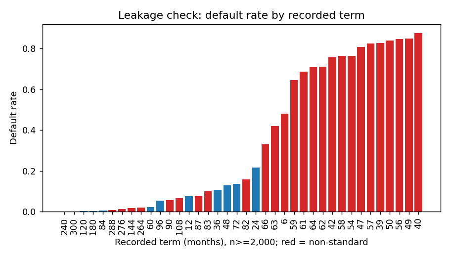
Term is excluded. The honest out-of-time AUC is 0.664.
Champion and challenger
Two models compete. The challenger baseline is a classic weight-of-evidence logistic scorecard, the kind a credit committee has seen for decades. The champion is a gradient-boosted model (LightGBM) with monotone constraints: predicted risk can only rise with the lender, industry and state charge-off rates, and only fall with employee count. Constraints keep the model defensible and usually more stable out of time. Each applicant also gets exact contribution-based reason codes, the format adverse-action notices need.
| Model (test: FY2006–07) | AUC | KS | Brier |
|---|---|---|---|
| WoE logistic scorecard | 0.616 | 0.19 | 0.278 |
| Monotone LightGBM (champion) | 0.664 | 0.24 | 0.237 |
AUC and KS measure ranking; Brier measures probability accuracy. Lower Brier is better.
The boosted model beats the scorecard in every single approval year from 1990 to 2007, not just on the pooled test set.
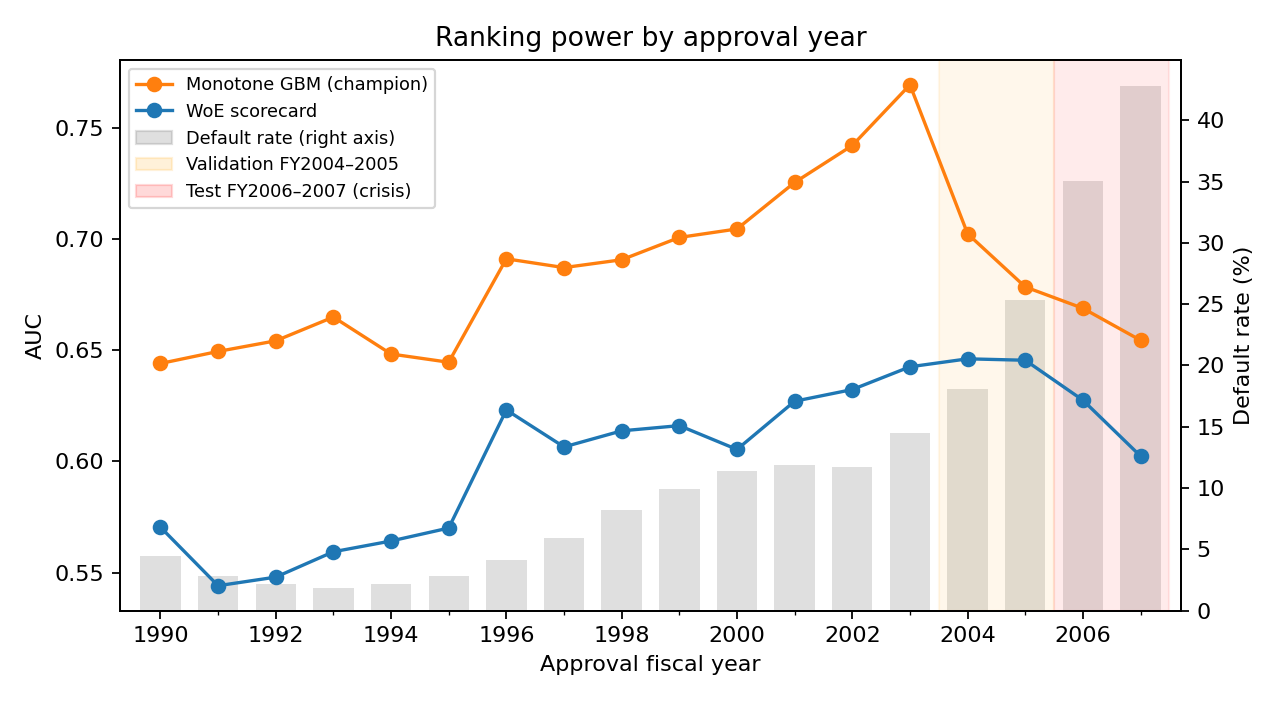
Ranking held. Calibration didn't.
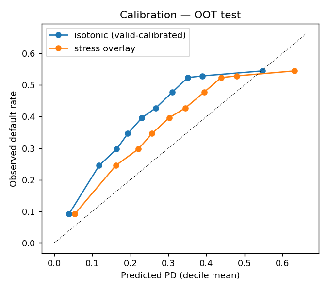
The model was calibrated on 2004–05, when defaults ran at 22%. In the crisis cohort, it predicted a mean default probability of 26% against 39% observed. Ranking held up; the level did not.
These are two different problems, and they need different fixes. I keep the ranking and shift the level with a stress overlay: a log-odds adjustment that moves the average predicted default rate to a stressed scenario (1.5 times the validation rate) without changing the order of any borrower. The scenario is set in advance, not taken from test outcomes. Calibration error falls from 0.128 to 0.077.
Loss given default: knowing when not to model
Four approaches competed for loss severity on defaulted loans: the portfolio average, a segment lookup, a fractional logit and a gradient-boosted model. None beat the portfolio average on validation by the 2% materiality bar I set in advance, and out of time every model's ranking of severity actually reversed: the crisis changed what drives losses.
So the pipeline uses the portfolio average, net of the SBA guarantee. Real lift in loss modeling needs collateral, lien position and cash-flow data at default, none of which this file has. Shipping a model that doesn't beat the average adds complexity and false precision.
From probability to price and policy
Probability of default becomes a decision through three steps:
- Expected loss = probability of default × loss given default × exposure.
- Risk-based rate = cost of funds + operating cost + capital charge + target margin + annualized expected loss. Across risk deciles, the indicated rate runs from about 8.8% to 13.6%.
- Approval cutoff is set on profit, not AUC. A profit curve finds the approval rate that maximizes illustrative lifetime profit.
The swap-set makes the improvement concrete. At the same 42.5% approval rate, the new model approves 14,687 loans the scorecard would have declined, with a 31% bad rate, and declines 14,687 the scorecard would have approved, with a 45% bad rate. That is where the profit comes from.
Recommendations
- Adopt the monotone boosted model as champion and keep the scorecard as challenger. It ranks better out of time and in every vintage, and stays explainable.
- Make leakage testing a standard validation step, and ban post-origination fields by data rule.
- Separate ranking from level. Recalibrate the intercept when the portfolio default rate moves, without retraining.
- Use portfolio-average loss, net of guarantee, until collateral data exists.
- Set cutoffs on profit and show the swap-set, so the business sees exactly which loans change decision.
- Retrain on recent vintages before any deployment. The score's population stability index between training and test is 1.64, far above the usual 0.25 review trigger, driven by program mix shifts such as SBA guarantee shares falling from about 85% to 59%.
Limits
The FOIA file contains only resolved loans, so recent vintages over-represent defaults; the test is read mainly as a ranking test. There is no bureau, cash-flow or collateral data, which caps discrimination near 0.66 AUC. That ceiling is the argument for cash-flow underwriting, which is the subject of the companion note, Fraud Is a Gate, Not a Feature.

Sources
Data
- U.S. Small Business Administration, 7(a) and 504 loan-level data, released under the Freedom of Information Act (public domain). Copy used: huggingface.co/datasets/MaddRaf/SBAnational
- Li, M., Mickel, A. and Taylor, S. (2018). "Should This Loan be Approved or Denied?: A Large Dataset with Class Assignment Guidelines." Journal of Statistics Education, 26(1). doi.org/10.1080/10691898.2018.1434342
Methods referenced
- Siddiqi, N. (2006). Credit Risk Scorecards: Developing and Implementing Intelligent Credit Scoring. Wiley.
- Ke, G. et al. (2017). "LightGBM: A highly efficient gradient boosting decision tree." Advances in Neural Information Processing Systems 30.
- Lundberg, S. M. et al. (2020). "From local explanations to global understanding with explainable AI for trees." Nature Machine Intelligence, 2, 56–67.
Independent research, not investment or lending advice; pricing parameters are illustrative. Analysis, code, charts and text were produced with AI assistance and reviewed by the author.