Every rates desk, bank treasury and insurer's ALM committee sees forecasts of the yield curve: from economists, vendors and, increasingly, machine-learning models. The decision is how much weight to give them when setting hedges and duration. The hard benchmark is the forecast that requires no model at all: next month's curve will look like today's.
I tested a deep-learning model (an LSTM network) and the standard factor model used in the literature against that benchmark, on daily US Treasury yields from 1990 to October 2026, forecasting at every month-end from January 2006 and refitting each model once a year on data known at the time.
Executive summary
The question. Should a forecast of the Treasury curve from a neural network, or from the standard factor model, drive hedging and duration decisions over the assumption that yields stay where they are?
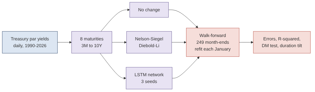
The approach. Eight maturities from 3 months to 10 years; 249 one-month and 247 three-month forecasts from January 2006 to October 2026; three models; annual refits with no look-ahead; error, out-of-sample R-squared, a Diebold-Mariano significance test and an illustrative duration-timing overlay.
The answer. "No change" is very hard to beat. The neural network matched it at the long end and improved on it by 4% to 5% at 3 months to 1 year, an improvement that is not statistically significant. The Nelson-Siegel factor model (Diebold-Li), which the academic literature often uses as the benchmark to beat, was 5% to 19% worse than no change at every maturity. Three months ahead, both models lost everywhere.
The decision. Treat any curve forecast, however sophisticated, as unproven until it beats no change out of sample, by maturity and horizon. Size hedges on the distribution of surprises, not on the point forecast.
Business outcomes
| Decision | What the data showed | What it means |
|---|---|---|
| Steer duration with the factor model | 5% to 19% more squared error than no change one month ahead; significantly worse at 2Y and 3Y (t = 2.2, 2.1) | The textbook model would have added error to every hedge decision |
| Steer duration with the neural network | 3.7% to 5.1% better at 3M–1Y, 0.1% to 0.8% worse at 5Y–10Y; best significance t = −1.45 | Indistinguishable from no change where duration risk lives |
| Time 10-year duration on the forecasts | LSTM +$41.0M over 249 months, Diebold-Li −$51.8M, at $100k per basis point; Sharpe-like ratios 0.22 and −0.28 | Neither result is distinguishable from luck over 21 years |
| Size risk on the surprise | One-month 10-year surprise of 26 bp in normal years, 44 bp in 2022 | $2.6M to $4.4M a month on a $100k-per-bp book |
| Use forecasts three months out | Both models worse than no change at every maturity | Longer horizons do not rescue the models |
Errors are root-mean-square, in basis points, of 249 one-month forecasts made at month-ends from January 2006 to September 2026. The duration overlay takes a long or short position each month on the sign of the 10-year forecast, sized at $100,000 per basis point (roughly $125M of 10-year notes), and counts yield moves only: no carry, roll or trading costs. Illustrative.
End to end in five steps
| Step | What happens | Output |
|---|---|---|
| 1. Source | Daily US Treasury par yields, January 1990 to October 2026 | Checksum-pinned public data |
| 2. Curve | Eight maturities complete since 1990: 3M, 6M, 1Y, 2Y, 3Y, 5Y, 7Y, 10Y | 9,211 trading days |
| 3. Models | No change; Nelson-Siegel factors with an autoregression per factor; an LSTM network reading the last 21 days | Three forecasters |
| 4. Walk-forward | Forecast at each month-end from January 2006; refit each January using only data known then | 249 one-month and 247 three-month forecasts |
| 5. Judge | Error by maturity, out-of-sample R-squared, Diebold-Mariano test, direction, duration overlay, sub-periods | Did any model beat no change? |
The data
US Treasury daily par yield curve, via the public defeatbeta Yahoo Finance mirror on Hugging Face (ODC-BY), pinned by checksum. I used the eight maturities with complete history since January 1990 and dropped the 1-month, 2-month and 20-year series, which start later or have gaps. Yields are in percent; forecast errors are in basis points.
The three forecasters
| Model | What it assumes | How it forecasts |
|---|---|---|
| No change (random walk) | Next month's curve equals today's | Nothing to fit |
| Nelson-Siegel factors (Diebold-Li) | The curve is a level, a slope and a curvature, and each drifts back toward its average | Fit the three factors each day; regress each factor's value h days ahead on today's; rebuild the curve |
| LSTM neural network | Recent daily moves and the curve's shape carry information about the next move | Read the last 21 days of the curve relative to today, plus today's level; predict the change in all eight yields; average three seeds |
The LSTM has one layer of 32 units, is trained with weight decay and stops early on the most recent 15% of its training window. At each annual refit, only training examples whose target date is on or before the refit date are used.
The results
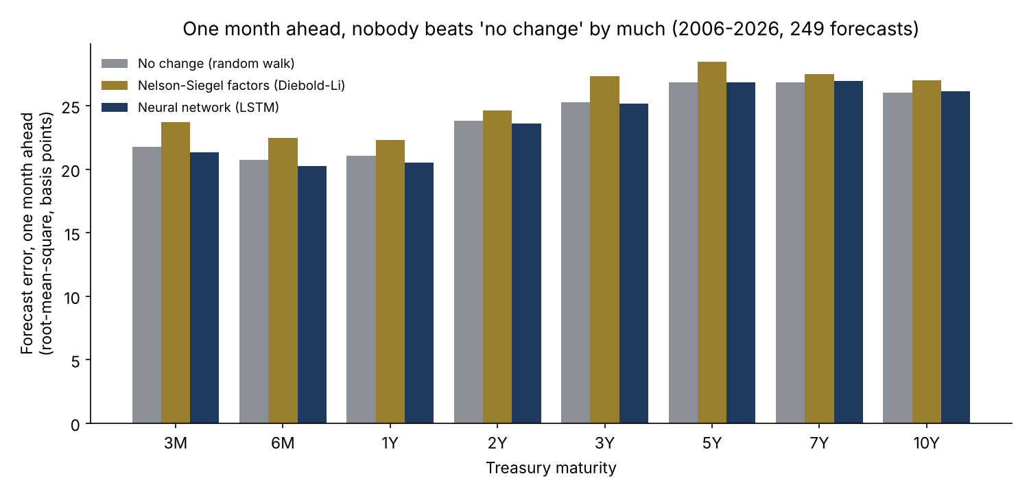
One month ahead, the three models sit within about two basis points of each other at every maturity. No change had a typical 10-year error of 26.0 bp, the LSTM 26.1 bp and Diebold-Li 27.0 bp.
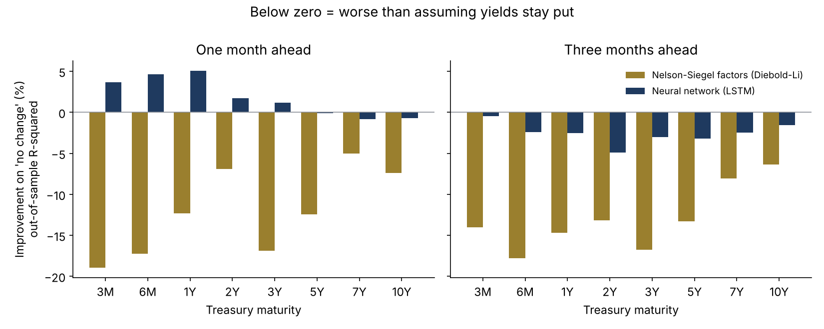
The neural network removed 3.7% to 5.1% of squared error at 3 months to 1 year, where yields are anchored by the policy rate and its recent path carries some information. At 5 to 10 years it was slightly worse. The Diebold-Mariano test cannot tell either result from zero: the best t-statistic is −1.45. The factor model was worse than no change at every maturity and horizon, and significantly worse at 2 and 3 years. Fitting three smooth factors and projecting each forward adds estimation error that, at a one-month horizon, outweighs whatever the factors' drift captures.
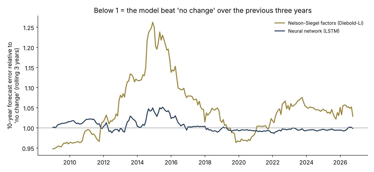
The factor model's worst stretch was the three years to 2015, when its 10-year error ran up to a quarter above no change. The network rarely strayed far from 1 in either direction, because it rarely forecast much at all: its typical forecast move was 2 to 4 bp, against actual monthly moves of 21 to 27 bp. Trained honestly, it learned that the best guess is close to no change.
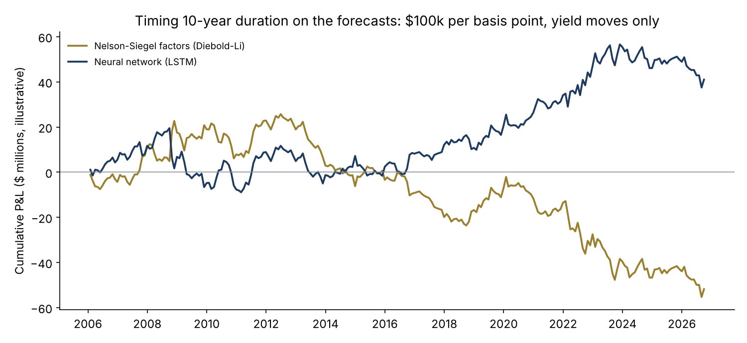
Accuracy and money are different questions. Because the overlay only uses the sign of the forecast, the network's small moves still called direction right 54% of the time at 10 years and made $41.0M over 249 months, mostly between 2017 and 2023, when yields trended. The factor model called direction right 44% of the time and lost $51.8M. With monthly swings of $2.6M, neither result is distinguishable from luck over 21 years.
| Period | No change, 10Y | LSTM, 10Y | Diebold-Li, 10Y | No change, 2Y | LSTM, 2Y | Diebold-Li, 2Y |
|---|---|---|---|---|---|---|
| 2006–2015 (120 months) | 26.6 | 26.9 | 27.4 | 21.8 | 21.6 | 23.2 |
| 2016–2026 (129 months) | 25.5 | 25.4 | 26.6 | 25.6 | 25.3 | 25.9 |
| 2022 hiking year (12 months) | 43.6 | 43.6 | 45.2 | 45.3 | 45.3 | 47.5 |
Root-mean-square one-month forecast error, basis points.
Recommendations
- Decision: adopt "beats no change out of sample, by maturity and horizon" as the minimum standard before any curve forecast, in-house or vendor, influences hedge ratios or duration targets.
- Controls: require walk-forward tests with no look-ahead, significance tests, and sub-periods that include 2022; reject results reported only in-sample or on one horizon.
- Hedging: size hedges on the distribution of surprises (26 bp typical, 44 bp in 2022 at 10 years) rather than on point forecasts.
- Where to look for value: the front end is the only place either model added accuracy. Test policy-path information there before reaching for more complex networks.
- Governance: re-test every forecast in use annually; retire any that fall below no change over the last three years.
Limits
- One market and one curve: US Treasury par yields. Results for swap curves or other countries may differ.
- The network is deliberately small and uses only the curve itself. Macro data, futures-implied policy paths or survey forecasts may add information; they are not tested here.
- 249 monthly forecasts is enough to rule out large gains, not small ones.
- The duration overlay ignores carry, roll-down and trading costs.
- Independent research on public data. Not deployed; not investment advice.
How it was built
Sources
- US Treasury daily par yield curve, via huggingface.co/datasets/defeatbeta/yahoo-finance-data (ODC-BY).
- Diebold, F. X. and Li, C. (2006). "Forecasting the Term Structure of Government Bond Yields." Journal of Econometrics 130(2).
- Nelson, C. R. and Siegel, A. F. (1987). "Parsimonious Modeling of Yield Curves." Journal of Business 60(4).
- Diebold, F. X. and Mariano, R. S. (1995). "Comparing Predictive Accuracy." Journal of Business & Economic Statistics 13(3).
- Campbell, J. Y. and Thompson, S. B. (2008). "Predicting Excess Stock Returns Out of Sample." Review of Financial Studies 21(4).
- Hochreiter, S. and Schmidhuber, J. (1997). "Long Short-Term Memory." Neural Computation 9(8).
Independent research on public data, not investment advice; dollar figures are illustrative. Analysis, code, charts and text were produced with AI assistance and reviewed by the author.