Can an LSTM Beat HAR? Deep Learning vs the Classic Volatility Model on 19 Years of S&P 500 Forecasts

Volatility forecasts sit under most of the decisions a risk function signs off:

how big a position may be;
how much value-at-risk a desk is using;
how much margin to call;
what an option is worth.

Risk teams are now being offered deep-learning models for this job. The pitch is that a neural network reading raw market history will find patterns the old models miss. The question for a risk committee is concrete: should it replace a proven model with one of these, and how would it know?

I tested this as a model-risk team would. The incumbents are HAR, a four-parameter regression that has been the academic standard for more than fifteen years, and the VIX, the volatility the options market prices. The challengers are two networks built in PyTorch: an LSTM and a temporal convolutional network (TCN), each reading 60 days of history. Every model was refit each January from 2008 to 2026 and scored on every day of the following year.

Watch: the walkthrough on Out of Sample.

0.325 vs 0.392

Forecast loss (QLIKE, lower is better): HAR + VIX against the LSTM, 4,688 out-of-sample days. The gap is significant at the 1% level

7 of 19

Years the LSTM beat HAR + VIX: all calm ones. It lost by 32% in 2008, 73% in 2018 and 25% in 2020

$38M

Deeper worst drawdown per $1bn when sizing a 15% volatility-targeted book with the LSTM instead of HAR

Weeks late

Every forecast in March 2020, the VIX included

Executive summary

The question. Can deep-learning sequence models forecast next-month S&P 500 volatility better than HAR and the VIX? Does any gain survive when the forecast is used to size a real book?

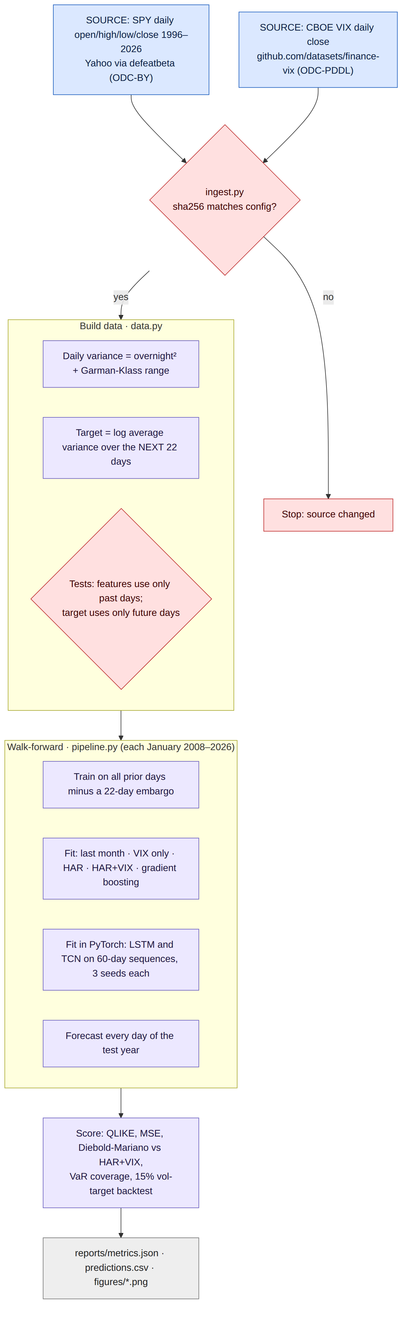
The approach. I built a daily variance estimate from SPY's open, high, low and close for 1996–2026, alongside the CBOE VIX. The target is average daily variance over the next 22 trading days. Seven forecasters were compared:

last month's realised volatility;
the VIX alone;
HAR;
HAR with the VIX and a leverage term;
gradient boosting on the same inputs;
an LSTM;
a TCN.

Every January from 2008 each model was refit on all earlier data, with a 22-day gap so no training target overlapped the test year. The networks were averaged over three random seeds, and nothing was tuned on the test years. Forecasts were scored with QLIKE and a Diebold–Mariano test. They were then put to work: sizing a 15% volatility-targeted S&P 500 book, and setting a 99% one-day VaR.

The answer. HAR plus the VIX had the lowest loss, and plain HAR was statistically tied with it. The LSTM's loss was 20% higher and the TCN's 38% higher, both significant. The networks won calm years and lost the crises, under-forecasting the most exactly when it mattered most. For sizing, every forecast roughly halved the index's drawdown. The simplest estimate kept the book closest to its target, and the LSTM was the worst of the forecasters.

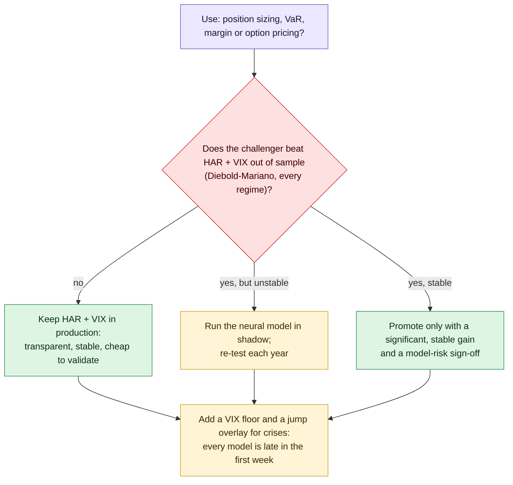
The decision it supports. Keep HAR plus the VIX as the production forecaster. Run neural models only as challengers in shadow, and promote one only on a significant, stable out-of-sample gain across regimes. Judge every forecaster by the decision it drives, not by its fit. Back all of them with a stress overlay, because none of them sees a crash coming.

Business outcomes

Decision	HAR + VIX	LSTM	What it means
Forecast loss (QLIKE), 2008–2026	0.325 (best)	0.392 (+20%; DM t = 2.6)	The challenger is worse, not just untested
Years better than the other	12 of 19	7 of 19, all calm	It loses when losses are largest
Average error when realised vol is above 30% (337 days)	13.6 points too low	19.0 points too low	A deeper under-call in exactly the days that matter
99% one-day VaR breaches (target 1%)	1.5%	2.0%	Both under-cover; the LSTM by more
15% vol-targeted book: worst drawdown	−32.6%	−34.2%	Buy and hold lost 53.0%
15% vol-targeted book: average yearly miss vs target	1.8 points	2.1 points	The trailing-month estimate was closest at 1.2
Compute for 19 annual refits	Seconds	About 36 minutes on 2 CPU threads (all models)	Cheap to test; costly to validate and govern

Out-of-sample, January 2008 to August 2026, 4,688 days. QLIKE uses realised next-month variance; DM = Diebold–Mariano with Newey–West errors. Vol-targeted book: SPY sized to 15% using each forecast, weekly rebalance, leverage cap 2, 2 bp per unit of turnover. Sizing with the LSTM rather than plain HAR deepened the worst drawdown from 30.3% to 34.2%, $38M per $1bn (illustrative).

End to end in five steps

Step	What happens	Output
1. Source	SPY daily open, high, low and close; CBOE VIX daily close; both checksum-pinned	30 years of daily data
2. Measure	Daily variance = overnight move squared + Garman–Klass range; target = average over the next 22 days	7,684 days with features and target
3. Fit	Each January from 2008, refit seven forecasters on all prior days, minus a 22-day gap; networks in PyTorch, three seeds each	19 refits per model
4. Score	QLIKE, MSE, Diebold–Mariano against HAR + VIX, year-by-year and stress-day errors	Which forecaster is better, and when
5. Use	Size a 15% volatility-targeted S&P 500 book; set a 99% one-day VaR	Drawdown, tracking to target, tail coverage

The data

SPY's daily open, high, low and close come from Yahoo Finance in a public mirror. The CBOE VIX comes from a public-domain copy of Cboe's own history file. Both files are pinned by checksum. The sample runs from March 1996 to September 2026. The out-of-sample test covers January 2008 to August 2026: 4,688 days, including the financial crisis, the 2015 and 2018 volatility shocks, COVID, the 2022 rate shock and the 2025 tariff selloff.

The models, in plain terms

Model	What it uses	How it learns
Last month	Average variance over the past 22 days	Nothing to fit: tomorrow looks like last month
VIX only	The options market's 30-day implied volatility	One regression coefficient
HAR	Variance yesterday, last week and last month	Linear regression: volatility has long memory
HAR + VIX	HAR plus the VIX plus recent negative returns (volatility rises more after falls)	Linear regression, seven coefficients
Gradient boosting	The same inputs as HAR + VIX	Hundreds of small decision trees
LSTM	The last 60 days of variance, VIX and returns, day by day	A recurrent network that carries a memory forward through the sequence
TCN	The same 60-day sequence	Stacked causal convolutions whose reach doubles at each layer

All forecasts target the log of next-month variance and are converted back with a bias correction estimated in training. The networks were trained in PyTorch on CPU with settings fixed before any results were seen.

What happened

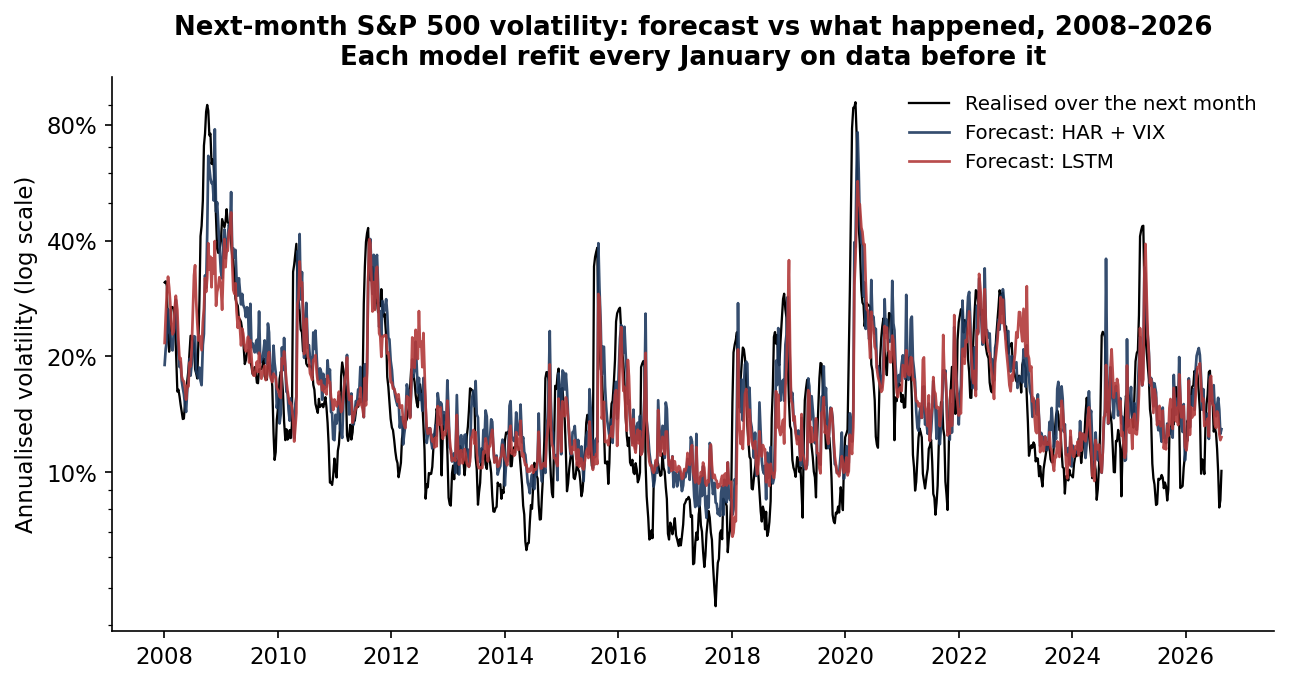
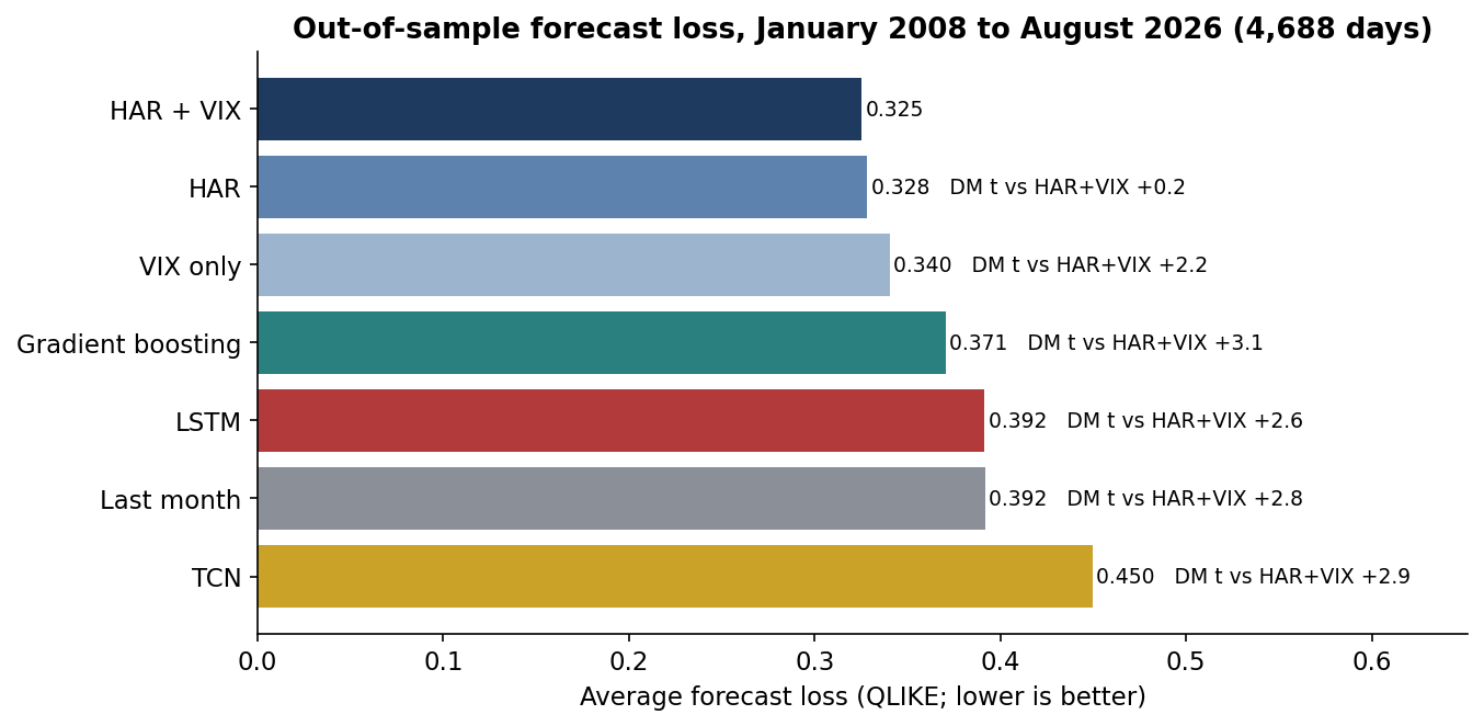
Line chart of realised next-month S&P 500 volatility against HAR plus VIX and LSTM forecasts, 2008 to 2026, log scale — Realised volatility over the following month (black) against the HAR + VIX and LSTM forecasts. Both track the regime. Both are late into every spike.

Horizontal bar chart of average QLIKE forecast loss for seven models with Diebold-Mariano statistics — Average out-of-sample loss. HAR + VIX is best; plain HAR is statistically tied. Every other model is significantly worse, the neural networks included.

Two results matter. First, the classic model was not just competitive; it was best. Adding the VIX and a leverage term to HAR made the forecast more accurate, but the gain over plain HAR was small and not significant. The VIX on its own was close behind. The networks, given more flexibility and the same information, did worse.

Second, the networks did not lose evenly. The LSTM beat HAR + VIX in seven years: 2009, 2013, 2014, 2016, 2019, 2024 and 2026 to date. Those are calm, trending years, when volatility drifts and memory is enough. It lost heavily in the stress years: by 32% in 2008, 18% in 2015, 73% in 2018 and 25% in 2020. On the 337 days when realised volatility was above 30%, it under-forecast by 19.0 points on average, against 13.6 for HAR + VIX.

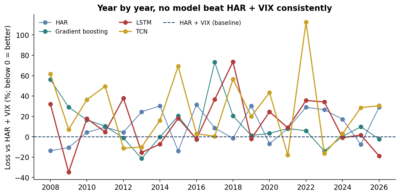
Line chart of each model's yearly forecast loss relative to HAR plus VIX, 2008 to 2026 — Loss relative to HAR + VIX, year by year (below zero means better). The networks' good years are calm years; their bad years are the shocks.

Why? Thirty years of daily data sounds like a lot, but the targets overlap. The effective sample is closer to 350 independent months, and only a handful of them are crises. A network has to learn volatility's long memory from scratch, while HAR is handed it as three numbers. In calm markets the network's extra flexibility fits small patterns. In a shock, it has seen too few to know how far volatility can go.

Line chart from January to June 2020 of realised next-month volatility against VIX, HAR plus VIX, LSTM and TCN forecasts — March 2020. Realised volatility over the following month (black) reached 90% while every forecast, including the VIX, sat near 20–30%. All of them caught up only after the damage was done.

Using the forecast

A forecast is only worth what the decision built on it is worth. I used each one to size an S&P 500 position to a 15% volatility target, rebalanced weekly, with leverage capped at two times and a small trading cost.

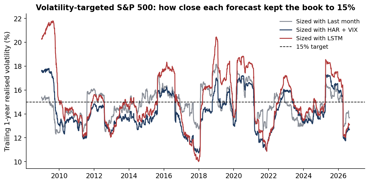
Trailing one-year realised volatility of the volatility-targeted book sized with last month, HAR plus VIX and LSTM forecasts, against a 15% target — How close each forecast kept the book to its 15% target, measured on a trailing year.

15% target book, sized with…	Return a year	Volatility	Sharpe	Worst drawdown	Average yearly miss vs 15%	99% VaR breach rate
Buy and hold (no target)	9.0%	19.8%	0.45	−53.0%	6.0 pts	n/a
Last month's realised	8.0%	14.8%	0.54	−28.0%	1.2 pts	2.0%
HAR	8.0%	14.5%	0.55	−30.3%	1.7 pts	1.7%
HAR + VIX	7.6%	14.3%	0.53	−32.6%	1.8 pts	1.5%
LSTM	7.9%	15.4%	0.51	−34.2%	2.1 pts	2.0%
TCN	8.2%	16.1%	0.51	−36.3%	2.0 pts	2.5%

SPY price returns, January 2008 to August 2026. VaR: one-day 99% from each forecast assuming normal returns; 1% is the target breach rate.

Any of the forecasts beat doing nothing: volatility targeting cut the worst drawdown from 53% to between 28% and 36% and lifted the Sharpe ratio. Among the forecasts, three points stand out.

The most accurate forecast was not the best sizing tool. The trailing-month estimate kept realised volatility closest to target and had the shallowest drawdown. It also reacts to realised volatility and nothing else, which is what a target book needs.
The neural forecasts sized worst. The LSTM deepened the worst drawdown by 3.8 points against plain HAR, $38M per $1bn.
No forecast covered the tails. A normal 99% VaR built on any of them was breached between 1.5% and 2.5% of the time. VaR needs a fat-tail or stress add-on whichever forecaster sits underneath.

The commercial case

The product here is not a better forecaster. It is a challenger lab: a standard, reproducible way to test any proposed volatility or risk model against a strong baseline before it reaches production. Model-risk rules already expect challengers, and risk teams are being pitched machine-learning models every week.

Element	What it is	Basis
Who pays	Model-risk and validation teams at banks and insurers; CROs at asset managers and hedge funds; volatility-targeting and risk-parity product teams	Budget holders: head of model risk, CRO, head of quant
The problem in dollars	$38M deeper worst drawdown per $1bn from sizing with the LSTM instead of HAR; on stressed days about $7.9M per $1bn of understated one-day VaR against HAR + VIX	Drawdown 34.2% vs 30.3%; 5.4 vol points ÷ √252 × 2.326
The product	A walk-forward challenger harness: embargoed refits, seed averaging, QLIKE and Diebold–Mariano, decision tests for sizing and VaR, and a validation report a committee can sign	This repository is the working prototype
Proof	7 models, 19 annual refits, 4,688 out-of-sample days, every number reproducible	Public code and data
Build vs buy	6–8 weeks to wrap the harness around a client's data and models with one quant and one engineer; today many teams validate model by model, by hand	Illustrative effort
Pricing logic	$40–80k per model validation, or $150k a year for a standing challenger service	Illustrative; small against one avoided $38M drawdown
What could stop adoption	Access to the client's models and data; independence requirements for validation	Mitigation: run inside the client's environment
How a client judges it	Models stopped before production, time to validate, VaR coverage, significance of any promoted gain	Reported per model

All prices and effort figures are illustrative assumptions with their arithmetic shown. Value figures come from this project's results; they are not a forecast for any firm.

The commercial point mirrors the risk point. The value is in the discipline that stops a weaker model reaching production, more than in any single clever model.

Recommendations

Keep HAR + VIX as the production volatility forecaster. It was the most accurate, it is transparent, and its handful of coefficients can be validated and explained to a committee.
Run neural models as shadow challengers. Re-test them each year on the same walk-forward design. Promote only on a significant gain that holds in stress years, not just on average.
Choose the forecaster by the decision. For volatility targeting, a responsive trailing estimate kept the book closest to target. For VaR and margin, a forward-looking input like the VIX matters more.
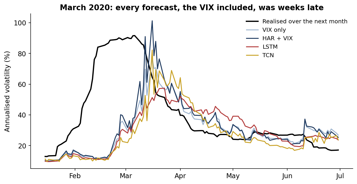
Put a stress overlay above every forecast. Every model was weeks late in March 2020. Add a VIX-jump trigger, a minimum volatility floor in sizing, and limits that do not depend on the model.
Add a fat-tail adjustment to VaR. Normal VaR on any of these forecasts breached 50% to 150% too often.
Govern neural models like any other model. Fix seeds and report the spread across them, keep the training window and embargo in code, and keep a strong simple baseline as the benchmark it must beat.

Limits

Daily data only. The variance measure comes from daily prices, not intraday trades. Neural networks may do better with intraday data or many assets at once; that needs its own pre-registered test.
One index, one horizon. The test covers the S&P 500 at a one-month horizon.
Settings fixed in advance. Network settings were not tuned on the test years. A tuned network might look better in a backtest, which is exactly what a validator should distrust.
Simplified backtest. The volatility-targeting test uses price returns and ignores dividends and financing.
Independent research. This is independent research on public data. It has not been deployed and is not investment advice.

Pipeline flowchart from SPY and VIX data through checksum verification, daily variance, walk-forward refits of seven models and scoring — The full pipeline. Blue: external sources. Lavender: code steps. Red: checks and gates.

Decision flowchart for choosing a production volatility forecaster with a challenger process and stress overlay — How a risk committee would choose and govern the forecaster.

Sources

Data

SPY daily open, high, low and close: Yahoo Finance. Copy used: huggingface.co/datasets/defeatbeta/yahoo-finance-data (ODC-BY).
CBOE Volatility Index (VIX), daily: Cboe Global Markets. Copy used: github.com/datasets/finance-vix, data/vix-daily.csv (ODC-PDDL-1.0), downloaded 28 October 2026.

Methods referenced

Corsi, F. (2009). "A Simple Approximate Long-Memory Model of Realized Volatility." Journal of Financial Econometrics, 7(2), 174–196. ideas.repec.org/a/oup/jfinec/v7y2009i2p174-196.html
Garman, M. B. and Klass, M. J. (1980). "On the Estimation of Security Price Volatilities from Historical Data." Journal of Business, 53(1), 67–78.
Hochreiter, S. and Schmidhuber, J. (1997). "Long Short-Term Memory." Neural Computation, 9(8), 1735–1780.
Bai, S., Kolter, J. Z. and Koltun, V. (2018). "An Empirical Evaluation of Generic Convolutional and Recurrent Networks for Sequence Modeling." arXiv:1803.01271.
Patton, A. J. (2011). "Volatility Forecast Comparison Using Imperfect Volatility Proxies." Journal of Econometrics, 160(1), 246–256.
Diebold, F. X. and Mariano, R. S. (1995). "Comparing Predictive Accuracy." Journal of Business & Economic Statistics, 13(3), 253–263.
Bucci, A. (2020). "Realized Volatility Forecasting with Neural Networks." Journal of Financial Econometrics, 18(3), 502–531. ideas.repec.org
Christensen, K., Siggaard, M. and Veliyev, B. (2023). "A Machine Learning Approach to Volatility Forecasting." Journal of Financial Econometrics, 21(5), 1680–1727. ideas.repec.org
Moreira, A. and Muir, T. (2017). "Volatility-Managed Portfolios." Journal of Finance, 72(4), 1611–1644. nber.org/papers/w22208

Code & downloads

View the code: lstm-vs-har-volatility (PyTorch)→Download the research note (PDF)↓

Independent research on public data, not investment advice; dollar figures are illustrative. Analysis, code, charts and text were produced with AI assistance and reviewed by the author.