Consumer instalment loans have become a mainstream holding for private credit funds, insurers and banks, bought through forward-flow agreements with lending platforms. The buyer is paid through the coupon, and the coupon rises with the platform's risk grade. A loan graded E pays nearly three times the rate of a loan graded A. The committee question is simple: did the higher coupon actually pay for the higher losses?
The answer matters now. Asset-based finance is one of the fastest-growing corners of private credit, and lenders are hiring senior credit-risk leaders to set prices, read vintages and decide when to stop buying. I tested the question on the one long, public, loan-by-loan record of a major US consumer lending platform: every 36-month loan LendingClub issued from 2007 to 2015, followed to the end of its term.
Executive summary
The question. For a buyer of consumer instalment loans: did the coupon at each risk grade cover the losses that followed? How early can a buyer tell that a new vintage is running worse than priced? And does screening loans inside each grade add return that holds up out of sample?
The approach. I took the 618,731 LendingClub 36-month loans ($7.7bn) that met the platform's credit policy, were issued from June 2007 to December 2015, and had all run to the end of their term by the March 2019 data cut. For each pool of loans I built month-by-month cash flows and measured the realised annual return a buyer earned after a 1% servicing fee. I then tracked each quarterly vintage's defaults by month on book, and forecast every vintage's final default rate using only the information available at the time. Finally, I trained a credit model on 2010–2013 loans, tuned it on 2014, and tested it once, on 2015.
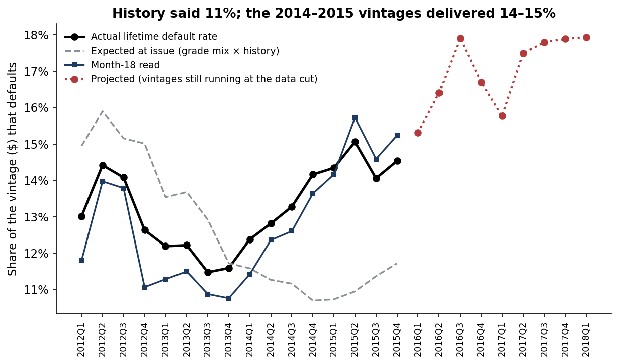
The answer. The coupon rose steadily with risk; the return did not. Realised returns peaked at grade B (7.0% a year) and fell to 2.4% for grade G. The extra coupon in the lowest grades was more than consumed by losses. The premium also eroded over time. Grades D and E returned 10–11% a year in the 2010–2013 vintages, but 3.4% and 0.7% in the 2015 vintage, below a 3-year Treasury for E. Pricing from seasoned history expected 11.2% of dollars in the 2014Q4–2015Q4 vintages to default; 14.4% did. A read of each vintage at month 18 was within 0.7 points of its final outcome. A model that screens inside each grade added 39 basis points a year, but could not rescue grades that were mispriced.
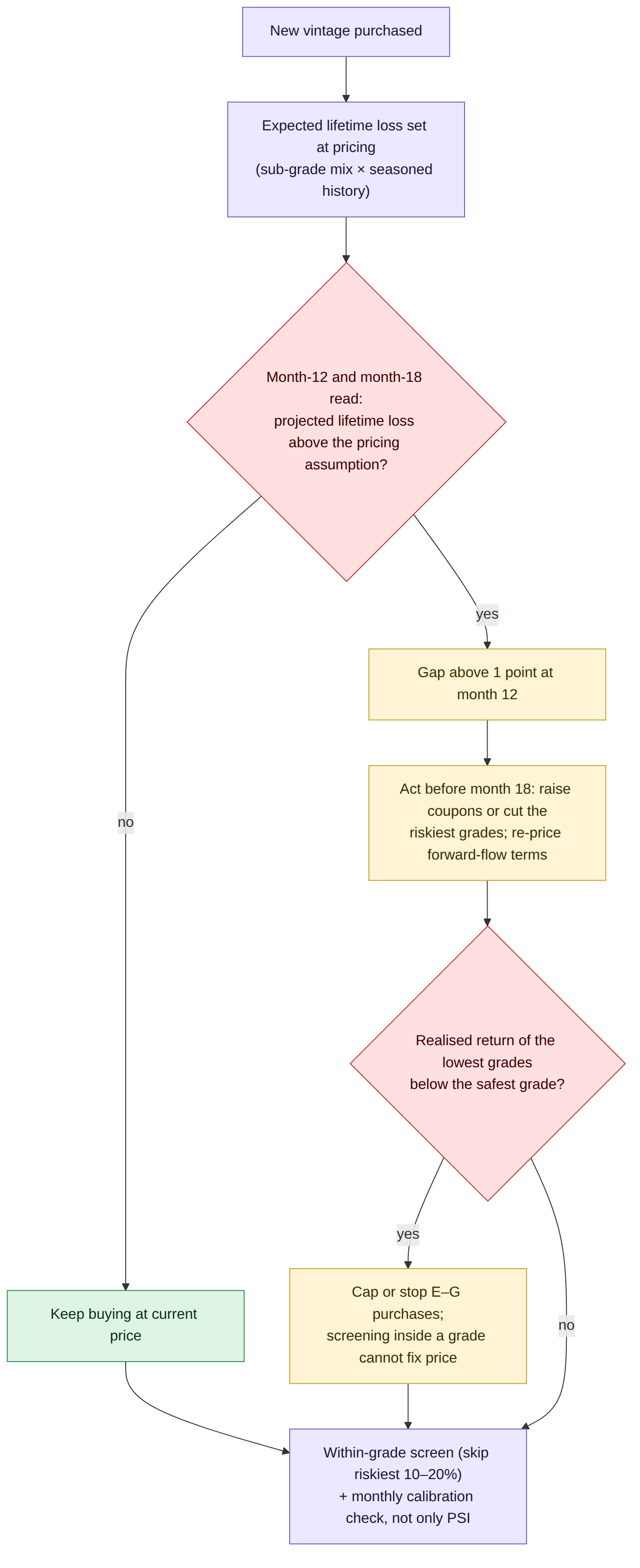
The decision it supports. Buy consumer credit on realised, risk-adjusted return by grade, not on coupon. Read every vintage at months 12 and 18 against its pricing assumption, and re-price or stop buying the lowest grades when the gap opens. Use within-grade screening as an addition to that discipline, never as a substitute for it. Monitor model calibration against outcomes, because the score's stability index will not warn you.
Business outcomes
| Business lever | What the buyer saw | What the evidence shows | What it means |
|---|---|---|---|
| Coupon vs return by grade | 7.2% (A) rising to 25.3% (G) | Realised 5.3% (A), 7.0% (B), 6.3% (D), 4.8% (E), 2.4% (G) | The best risk-adjusted return sat in the middle grades |
| Lowest grades, by vintage | D and E paid 10.1% and 11.0% (2010–2013) | 2015 vintage: D 3.4%, E 0.7%, F −3.4% | A premium that worked for four years disappeared in two |
| Pricing assumption, 2014Q4–2015Q4 | 11.2% of dollars expected to default | 14.4% defaulted | About $17M of extra net loss per $1bn bought |
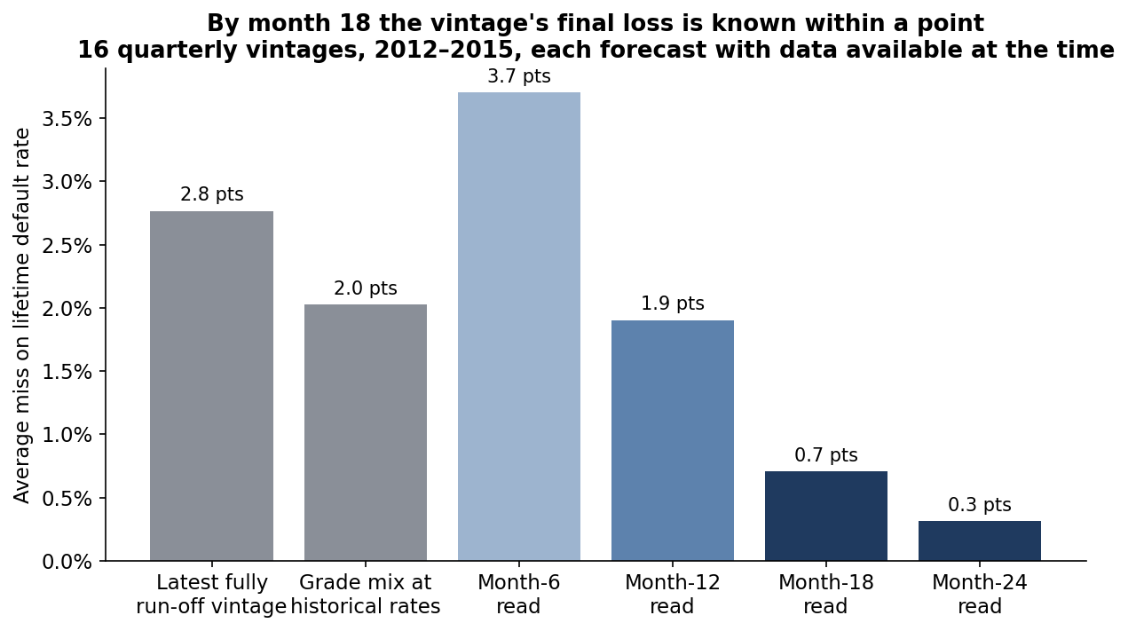
| Knowing early | Wait for vintages to run off (3+ years) | Month-12 read within 1.9 points; month-18 within 0.7 | A pricing decision 18 months in, not 40 |
| Screening inside each grade | Buy every loan in the grade | Skip riskiest 20%: 4.79% → 5.19% a year (2015) | About $3.9M a year per $1bn kept |
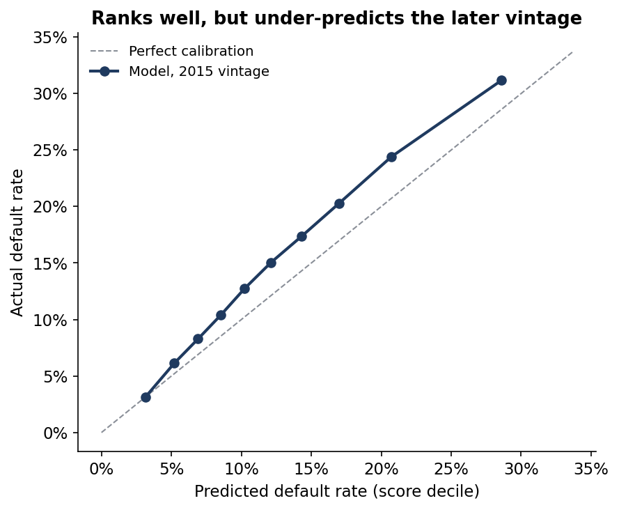
| Model monitoring | Score stability index 0.006 (no alert) | Default rate under-predicted by 2.2 points | Stability checks miss outcome drift |
Realised return: internal rate of return of pooled monthly cash flows after a 1% servicing fee, recoveries net of collection fees. Extra net loss = 3.27-point default gap × 51.7% net loss per defaulted dollar × $1bn. Screen value = 0.39 points × $1bn. Dollar figures are illustrative.
End to end in five steps
| Step | What happens | Output |
|---|---|---|
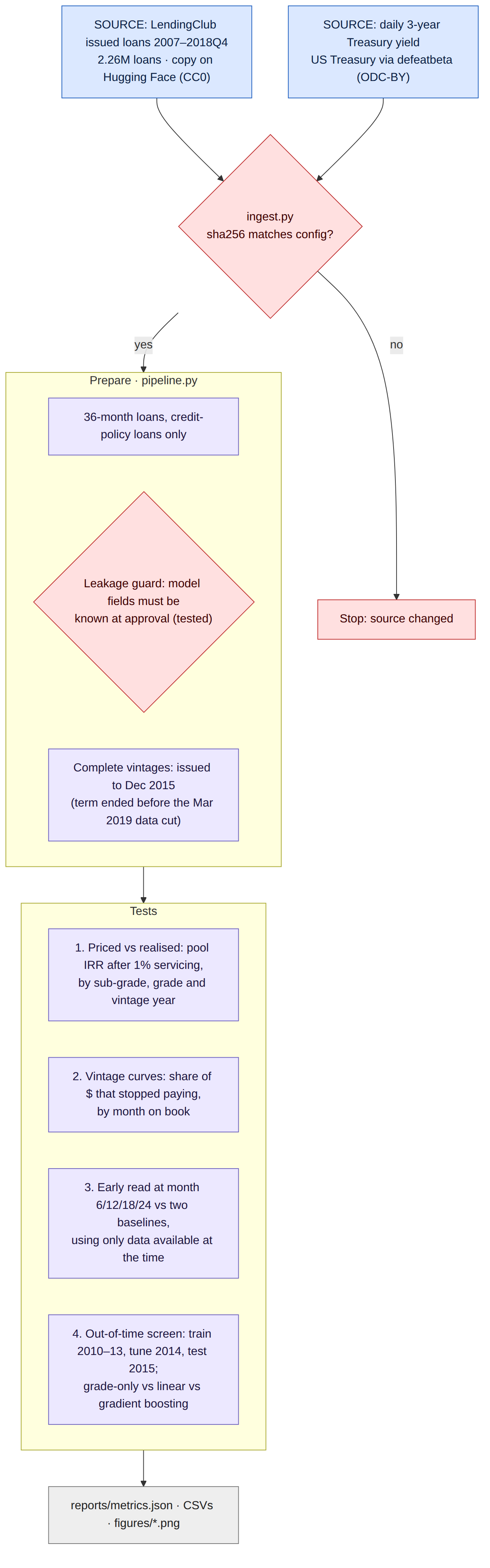
| 1. Source | LendingClub's issued-loan file (2.26M loans, 2007–2018) and the daily 3-year Treasury yield; both pinned by checksum | Raw data with provenance |
| 2. Clean | 36-month loans that met credit policy; default = charged off, in default or 31–120 days late; complete = term ended before the data cut | 618,731 complete loans, 1.6M in total |
| 3. Return | Monthly cash flows per pool: purchase, borrower payments less a 1% fee, recoveries six months after the last payment; internal rate of return | Realised return by grade, sub-grade and vintage |
| 4. Vintages | Share of each quarterly vintage's dollars that stopped paying, by month on book; forecasts at months 6–24 using only data available then | How early the outcome is knowable |
| 5. Screen | Model trained 2010–2013, tuned 2014, tested once on 2015; skip the riskiest 10% or 20% inside each sub-grade; random skip as control | Out-of-sample value of selection |
The data
The loan file is the platform's own public record of every loan it issued from 2007 to the end of 2018: 2.26 million loans, with the terms at origination, the borrower's credit attributes at application, and the payment history summarised at the March 2019 data cut. I used a public copy on Hugging Face, released under CC0, that matches the widely used compilation of the platform's files.
Three rules keep the comparison honest:
- Only complete loans are scored for returns. A 36-month loan issued by December 2015 has run its full term by the data cut, so its outcome is final. Later vintages are used only for the forward-looking projection.
- Only application data enter the model. Payment amounts, recoveries, later credit-bureau pulls, hardship and settlement flags are all observed after the loan is made. A test enforces that none can reach the model.
- The buyer's economics are stated. Returns are after a 1% servicing fee, the platform's published investor fee, and before funding costs.
How the return is measured
| Term | Meaning | Why it matters |
|---|---|---|
| Coupon | The promised interest rate on the loan | What the buyer is told it will earn |
| Realised return | The annual internal rate of return on the cash the pool actually paid back | What the buyer did earn, after defaults, prepayments and recoveries |
| Default (stopped paying) | Charged off, in default, or 31–120 days late at the data cut | The event that turns coupon into loss |
| Net loss | Funded principal not repaid, less recoveries net of collection fees | 51.7 cents per defaulted dollar across the sample |
| Vintage | All loans issued in the same quarter | The unit buyers price, monitor and re-price |
| Month on book | Months since the loans were issued | Where on its life cycle a vintage is |
The file records totals, not each month's payment, so the cash flows spread each loan's payments evenly from the first month to its last payment, with recoveries six months later. That blurs the timing of prepayments but is applied identically to every pool compared. Moving recoveries to three or twelve months changes grade returns by at most 0.06 points.
The coupon rose with risk; the return did not
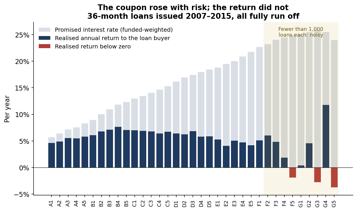
| Grade | Loans | Promised rate | Dollars that defaulted | Net loss | Realised return | Over 3-year Treasury |
|---|---|---|---|---|---|---|
| A | 142,925 | 7.2% | 5.2% | 2.4% | 5.3% | +4.5 pts |
| B | 211,692 | 10.8% | 11.0% | 5.3% | 7.0% | +6.1 pts |
| C | 161,843 | 13.9% | 17.9% | 9.3% | 6.8% | +5.9 pts |
| D | 76,074 | 17.2% | 24.0% | 13.4% | 6.3% | +5.4 pts |
| E | 21,410 | 19.8% | 29.8% | 17.5% | 4.8% | +3.9 pts |
| F | 4,265 | 23.5% | 35.5% | 21.9% | 4.1% | +3.2 pts |
| G | 522 | 25.3% | 38.4% | 24.7% | 2.4% | +1.5 pts |
36-month loans issued June 2007 to December 2015, all fully run off. Rates and default shares are weighted by funded dollars. Treasury = 3-year yield at issue, dollar-weighted.
Going from grade B to grade E added 9 points of coupon and 19 points of default. Losses absorbed all of the extra rate and more, and the realised return fell by 2.2 points. Every grade still beat Treasuries over the full period, but the spread a buyer earned per unit of risk was best in grades B and C.
The premium disappeared
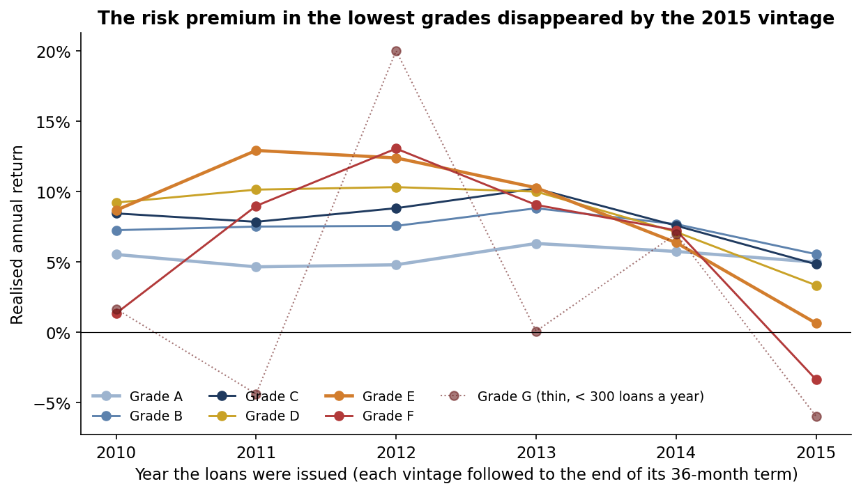
The full-period averages hide a reversal. Loans issued from 2010 to 2013 behaved as a buyer would hope: grade D returned 10.1% a year and grade E 11.0%, against 5.7% for grade A. In the 2014–2015 vintages, D returned 4.8% and E 2.9%. Loans issued in 2015 alone returned 3.4% (D), 0.7% (E) and −3.4% (F). Coupons did not rise to match: the average rate on new loans fell from 12.7% in early 2014 to 10.7% by the end of 2015.
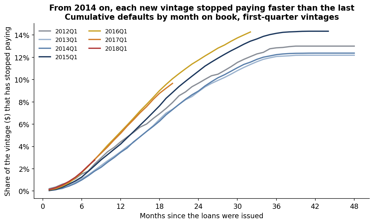
How early could a buyer have known?
A vintage's final loss is not known for more than three years. A buyer pricing new loans needs an earlier read. The standard approach is to take how much of the vintage has stopped paying at a given month and scale it up by the development seen in older, fully run-off vintages, the same chain-ladder logic insurers use to reserve claims. I tested it on 16 quarterly vintages from 2012 to 2015. Each forecast used only the vintages that had fully run off by the forecast date.
| Forecast made | Using | Average miss |
|---|---|---|
| At issue | The latest fully run-off vintage's default rate | 2.8 pts |
| At issue | Sub-grade mix × default rates of run-off vintages (the pricing assumption) | 2.0 pts |
| Month 6 | Defaults so far × development factor | 3.7 pts |
| Month 12 | Defaults so far × development factor | 1.9 pts |
| Month 18 | Defaults so far × development factor | 0.7 pts |
| Month 24 | Defaults so far × development factor | 0.3 pts |
16 quarterly vintages, 2012Q1–2015Q4; lifetime default share of funded dollars. Development factors are dollar-weighted over vintages that had fully run off by the forecast date.
Month 6 is too early: so few loans have stopped paying that small differences get magnified. By month 12 the read matches the pricing assumption; by month 18 it is three times as accurate. For the 2014Q4–2015Q4 vintages, the pricing assumption said 11.2%, the month-12 read said 13.6%, the month-18 read said 14.8%, and the outcome was 14.4%.
Does screening inside a grade help?
The platform's grade is its own risk score, and the coupon is set from it. A buyer can still choose which loans in each grade to take. I trained a gradient-boosted model on application data for loans issued in 2010–2013, early-stopped it on 2014, and scored the 2015 vintage once. The baselines were the grade alone and a linear scorecard on the same inputs.
| Model (test: 283,173 loans issued in 2015) | AUC | AUC within sub-grade | Brier score | Pool return, skip riskiest 20% in each sub-grade |
|---|---|---|---|---|
| Sub-grade only (the platform's price) | 0.678 | 0.500 | 0.1218 | 4.79% (buy everything) |
| Linear scorecard | 0.678 | 0.564 | 0.1214 | 5.05% |
| Gradient-boosted model | 0.685 | 0.572 | 0.1205 | 5.19% |
| Random skip (control) | n/a | n/a | n/a | 4.80% |
AUC measures how well the score ranks defaulters above non-defaulters (0.5 = chance). Within-sub-grade AUC is the average inside each of the 35 sub-grades, weighted by loan count. Brier score: lower is better.
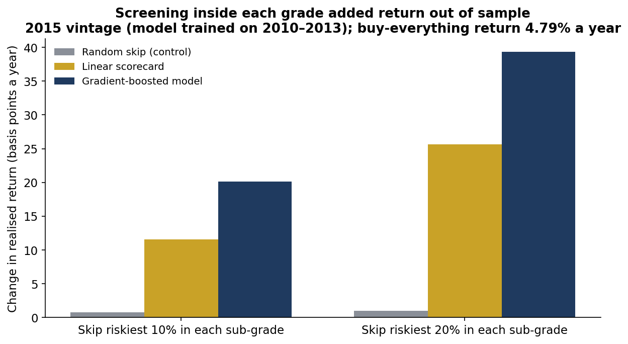
The model adds information the grade does not hold. Inside each sub-grade it ranks defaulters better than chance, using income, FICO, payment burden and loan purpose. Skipping the riskiest fifth of each sub-grade cut net loss by 0.54 points and raised the return by 39 basis points. Two limits matter as much as the gain. Screening did not rescue the lowest grades: after screening, the 2015 E, F and G loans still returned 1.0%, −2.9% and −4.6%. The problem there was price, not selection. And the model, trained on 2010–2013, predicted a 12.7% default rate for 2015 when 14.9% of loans defaulted.
The commercial case
The analysis is the prototype of a product that every buyer of consumer loans needs and few run well: a monthly vintage monitor with re-pricing triggers, plus a within-grade screen. The value comes straight from the results.
| Element | What it is | Basis |
|---|---|---|
| Who pays | Credit funds, insurers and banks buying consumer loans through forward-flow agreements; the capital-markets teams at lending platforms that must keep those buyers | Budget holders: head of asset-based finance, portfolio manager, chief risk officer |
| The problem in dollars | About $17M of extra net loss per $1bn bought when pricing drifts as it did in 2014–2015 | 3.27-point default gap × 51.7% severity |
| The product | Monthly vintage reads against the pricing plan, re-pricing triggers, a within-grade screen and a calibration report, delivered from the servicer's loan tape | This repository is the working prototype |
| Proof | Month-18 read within 0.7 points of the final default rate; screen +39 bp a year out of sample (band 36–42) | 2012–2015 vintages; 2015 test year |
| Value to a $1bn-a-year buyer | About $3.9M a year from screening, plus up to $16.9M per $1bn re-priced when a drift is caught | Base case, catching a quarter of one drift: about $8.2M a year |
| Build vs buy | 10–12 weeks for one quant and one data engineer: tape connectors, monitoring, model documentation. Today most buyers rely on analyst spreadsheets and the platform's own reports | Illustrative effort |
| Pricing logic | Under 5% of base-case value: monitor $150k a year; monitor plus screen $300k a year; or build-and-transfer at $250k with $75k a year of support | Illustrative; $300k is 3.7% of $8.2M |
| What could stop adoption | Access to loan tapes; validation on one platform only; a regime change that alters curve shape | Mitigation: pilot on one programme with a back-test on its own history |
| How a client judges it | Points of pricing gap caught, months to signal, basis points added, false-trigger rate | Reported monthly |
All prices and adoption assumptions are illustrative and shown with their arithmetic. Value figures come from the project's own results; they are not a forecast for any specific firm.
The commercial point is the same as the credit point: the money is in acting early. A buyer that reads its vintages at month 18 and has the right to re-price is buying an option worth millions per billion; a buyer that waits for run-off has already paid for the mistake.
Recommendations
- Set grade limits on realised, risk-adjusted return, not coupon. Over 2007–2015 the middle grades earned the best return per unit of risk. Cap the lowest grades and require a stated loss budget before buying them.
- Read every vintage at months 12 and 18 against its pricing assumption. At month 18 the read was within 0.7 points of the final outcome on average. If the projected lifetime loss runs more than one point above plan, review the coupon or the grade limits before the next purchase.
- Write the re-pricing trigger into forward-flow agreements. A buyer that can only respond after a vintage runs off is three years late. The 2014Q4–2015Q4 gap was about $17M of net loss per $1bn.
- Use within-grade screening as an overlay. It added about 40 basis points a year out of sample, but it cannot fix a grade that is priced too low.
- Monitor calibration against outcomes, not only score stability. The score's stability index stayed at 0.006 while the default rate ran 2.2 points above prediction. Compare predicted and actual defaults by vintage every month, and re-fit when they diverge.
- Govern the model like a credit policy. Restrict inputs to application data, test on a later year that was never used for tuning, and keep a random-skip control so the measured gain is not luck.
Limits
- One platform, one regime. These are unsecured US instalment loans from one marketplace with one grading system. The period from 2010 to 2018 had no recession, so these results do not describe a downturn.
- Approximate payment timing. Prepayment timing is approximated because the file holds totals, not monthly payments.
- Costs left out. Returns exclude funding costs, taxes and fees beyond the 1% servicing fee. Whole-loan and fractional buyers faced different terms.
- Approved loans only. Only funded loans are visible, so the screen ranks within the approved book and says nothing about declined applicants.
- Thin grades. Grades F and G are small: 4,265 and 522 complete loans.
- Independent research. This is independent research on public data. It has not been deployed and is not investment or lending advice.
Sources
Data
- LendingClub Corporation, issued-loan data 2007–2018Q4 (accepted loans), as published by the platform. Copy used: huggingface.co/datasets/codesignal/lending-club-loan-accepted, file accepted_2007_to_2018Q4.csv (CC0-1.0), downloaded 27 October 2026.
- US Department of the Treasury, daily par yield curve rates (3-year). Copy used: huggingface.co/datasets/defeatbeta/yahoo-finance-data (ODC-BY).
Methods and prior work referenced
- Emekter, R., Tu, Y., Jirasakuldech, B. and Lu, M. (2015). "Evaluating credit risk and loan performance in online Peer-to-Peer (P2P) lending." Applied Economics, 47(1), 54–70. ideas.repec.org/a/taf/applec/v47y2015i1p54-70.html
- Serrano-Cinca, C., Gutiérrez-Nieto, B. and López-Palacios, L. (2015). "Determinants of Default in P2P Lending." PLoS ONE, 10(10), e0139427. doi.org/10.1371/journal.pone.0139427
- Breeden, J. L. (2007). "Modeling data with multiple time dimensions." Computational Statistics & Data Analysis, 51(9), 4761–4785. ideas.repec.org/a/eee/csdana/v51y2007i9p4761-4785.html
- Mack, T. (1993). "Distribution-free calculation of the standard error of chain ladder reserve estimates." ASTIN Bulletin, 23(2), 213–225. casact.org abstract
- Ke, G. et al. (2017). "LightGBM: A highly efficient gradient boosting decision tree." Advances in Neural Information Processing Systems 30.
- Siddiqi, N. (2006). Credit Risk Scorecards: Developing and Implementing Intelligent Credit Scoring. Wiley.
Independent research on public data, not investment or lending advice; dollar figures are illustrative. Analysis, code, charts and text were produced with AI assistance and reviewed by the author.