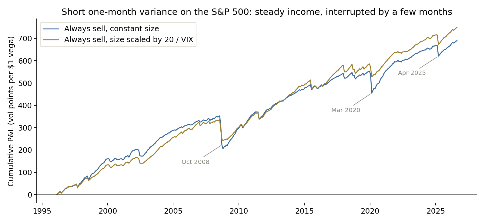
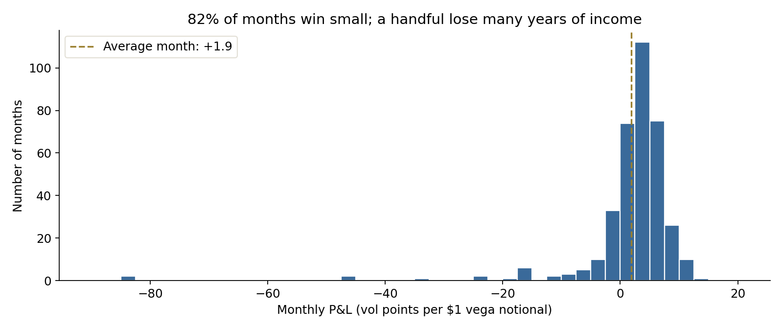
Investors pay up for protection against an equity crash, and someone is paid to provide it. Over thirty years of real data, the seller of one-month S&P 500 volatility made money in 82% of months. The worst month, October 2008, cost about 44 average months of that income in one go, and March 2020 cost almost as much.
The question for a committee is not whether the volatility premium exists. It does. The question is how much of it to own, sized so that the month it fails is survivable.
Executive summary
The question. What has selling S&P 500 crash insurance actually earned after costs, what does the bill look like when it comes due, and how large a position can a committee justify?
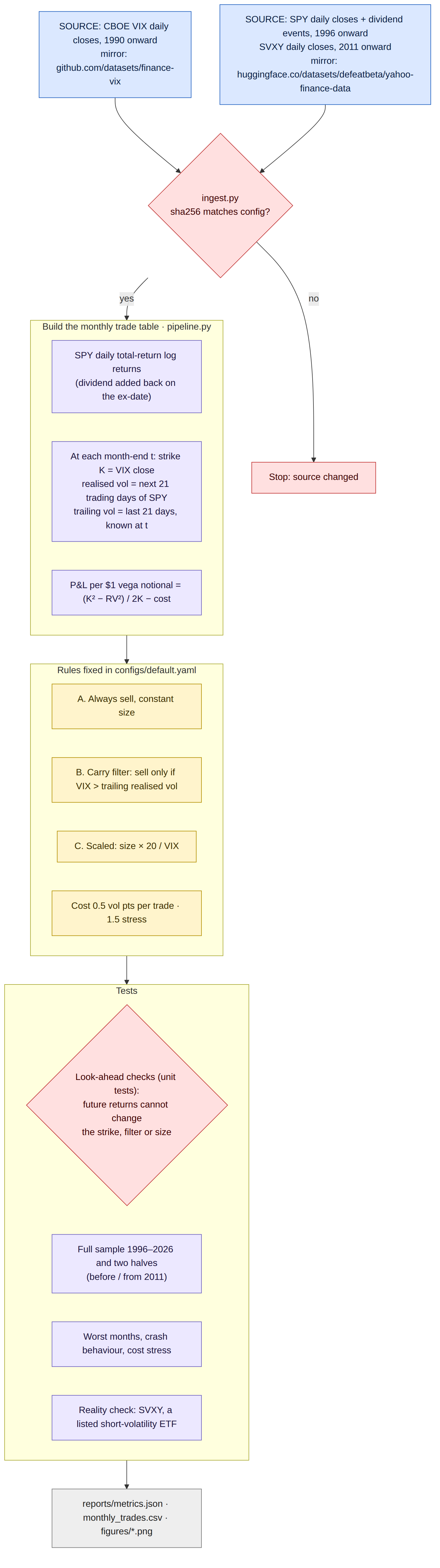
The approach. Each month-end from February 1996 to August 2026, sell one month of S&P 500 variance at the VIX level, the market's price for the next month's volatility, and settle it against the volatility that actually followed. That is 365 trades on real public data, with an illustrative cost per trade. Three rules were fixed before any result was seen: always sell at constant size; sell only when implied volatility exceeds recent realised volatility; and always sell, but scale the size down when VIX is high. A listed short-volatility ETF serves as a reality check.
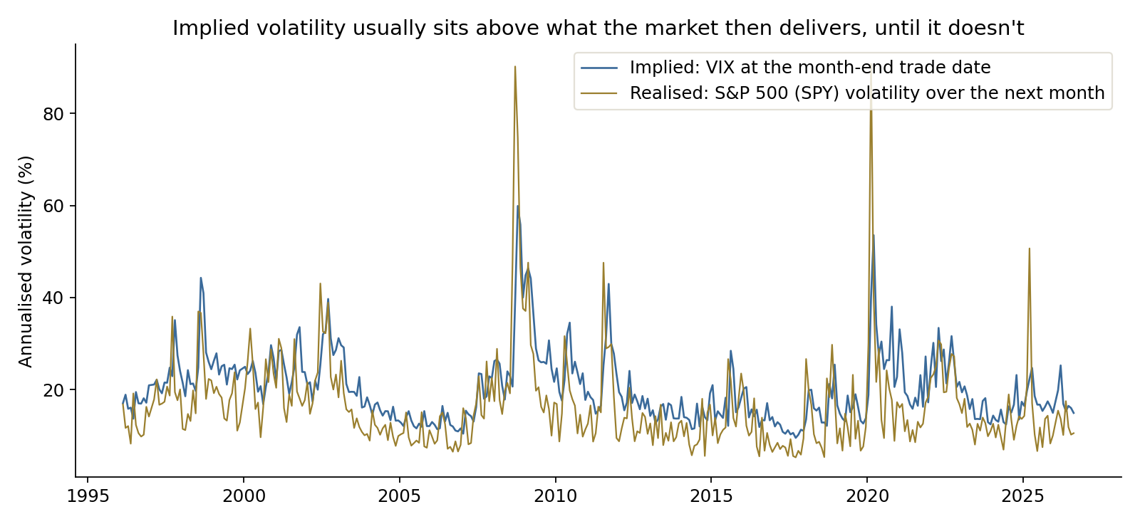
The answer. The premium is real: implied volatility exceeded the volatility that followed in 83% of months, by 3.8 points on average. After costs the constant-size trade earned about 1.9 vol points a month per dollar of vega with a Sharpe ratio of 0.72, but with a skew of -5.9. Scaling the position by 20 divided by VIX halved the worst month and raised the Sharpe ratio to 0.98, and it held in both halves of the sample. Filtering on recent volatility did not remove the tail.
The decision it supports. Own the premium only at a size where the worst month on record costs a stated, survivable share of capital, scale exposure down as volatility rises, and stress-test against a month twice as bad as anything in the data.
Business outcomes
| Dimension | Constant size | Size × 20 / VIX | What it means |
|---|---|---|---|
| Average monthly P&L (vol points per $1 vega) | +1.89 | +2.06 | Similar income from the two rules |
| Sharpe ratio, 1996–2026 | 0.72 | 0.98 | Scaling improves the return per unit of risk |
| Worst month (month of exposure) | -84.1 (Oct 2008) | -44.8 (Sep 2008) | Scaling halves the tail |
| Worst month in average months of income | 44 | 22 | How long one bad month takes to earn back |
| Vega notional on $1bn, worst month = 5% of NAV | $0.59M per vol point | $1.12M per vol point at VIX 20 | Size set by the tail, not by the average |
| Expected premium per year on $1bn | $13.5M (1.35%) | $27.6M (2.76%) | Same worst-case budget, about twice the income |
| A month twice the worst on record | -$100M (-10% of NAV) | -$100M (-10% of NAV) | The stress the committee must accept either way |
| Sharpe ratio at 1.5 vol points of cost | 0.34 | 0.45 | Execution cost decides whether it is worth doing |
P&L per $1 of vega notional, after an illustrative 0.5 vol-point cost per trade unless stated. Dollar figures apply the measured results to an illustrative $1bn portfolio: vega notional = 5% × $1bn ÷ worst month; expected premium = 12 × average month × vega notional.
End to end in five steps
| Step | What happens | Output |
|---|---|---|
| 1. Source | CBOE VIX daily closes (1990 onward); SPY daily closes and dividends (1996 onward); SVXY daily closes (2011 onward); every file checksum-pinned | Raw data with provenance |
| 2. Build trades | At each month-end, strike = VIX close; realised volatility = next 21 trading days of SPY total returns | 365 monthly trades |
| 3. Apply rules | Always sell; carry filter; size × 20 / VIX; 0.5 vol-point cost, 1.5 in the stress test | Monthly P&L per rule |
| 4. Test | Full sample, two halves, worst months, crash behaviour, cost stress, listed-ETF reality check, look-ahead unit tests | Performance and tail statistics |
| 5. Translate | Size each rule so the worst month costs 5% of an illustrative $1bn; then a month twice as bad | Committee sizing table |
The data
VIX is the CBOE's estimate of the market's expected S&P 500 volatility over the next 30 days, calculated from a strip of index options. It is constructed to approximate the rate at which a one-month variance swap would trade, which makes it the natural strike for this test. Realised volatility comes from SPY, the largest S&P 500 ETF, with dividends added back on the ex-date. SVXY, an ETF that sold short-dated VIX futures, shows what happened to investors who held a listed version of the same exposure.
The trade, in plain terms
A one-month variance swap pays the difference between the variance agreed at the start and the variance the market actually delivers. The seller is paid when the market turns out calmer than priced and pays out when it turns out wilder. Expressed per dollar of vega notional, the monthly result is (strike² − realised²) ÷ (2 × strike), in volatility points.
| Term | Definition used here |
|---|---|
| Strike | VIX close on the last trading day of the month |
| Realised volatility | Annualised volatility of the next 21 daily SPY total returns, measured as a variance swap pays (no mean subtracted) |
| Vega notional | Dollars gained or lost per volatility point, near the strike |
| Carry filter | Trade only if VIX exceeds the realised volatility of the previous 21 days |
| Scaled size | Vega notional multiplied by 20 ÷ VIX at the trade date |
| Cost | 0.5 vol points per trade, illustrative; 1.5 in the stress test |
Everything is known on the trade date: the strike, the filter and the size. Unit tests change every return after the trade date and confirm that none of them move.
What it paid, and what it cost
| Worst months, constant size | P&L (vol points) | VIX at the trade | Volatility that followed | S&P 500 (SPY) that month |
|---|---|---|---|---|
| October 2008 | -84.1 | 39.4 | 90.2 | -19.8% |
| March 2020 | -83.1 | 40.1 | 90.8 | -11.1% |
| April 2025 | -47.0 | 22.3 | 50.7 | -0.9% |
| September 2008 | -46.2 | 20.7 | 48.1 | -9.4% |
| August 2011 | -32.7 | 25.3 | 47.6 | -6.2% |
| July 2002 | -24.3 | 25.4 | 43.1 | -8.1% |
Month of exposure; each trade is struck at the close of the prior month. April 2025 shows that the loss is driven by volatility, not by the index level: the S&P 500 ended the month almost flat after a violent round trip.
Three findings matter for a decision. First, the trade is a disguised equity exposure: its monthly P&L has a correlation of 0.56 with the S&P 500, and in the ten worst months for the index it lost 26.6 points on average while the index fell 12.1%. Second, the losses cluster in the worst moment for the rest of a portfolio. Third, the carry filter did not help where it mattered: it skipped October 2008 but still sold into March 2020, and its Sharpe ratio fell from 1.23 before 2011 to 0.54 after.
| Rule | Before 2011: Sharpe / worst month | From 2011: Sharpe / worst month |
|---|---|---|
| Always sell, constant size | 0.76 / -84.1 | 0.68 / -83.1 |
| Carry filter | 1.23 / -46.2 | 0.54 / -83.1 |
| Size × 20 / VIX | 1.02 / -44.8 | 0.96 / -42.2 |
The scaled rule is the only one whose tail and return per unit of risk are stable across both halves.
The reality check: a listed short-volatility fund
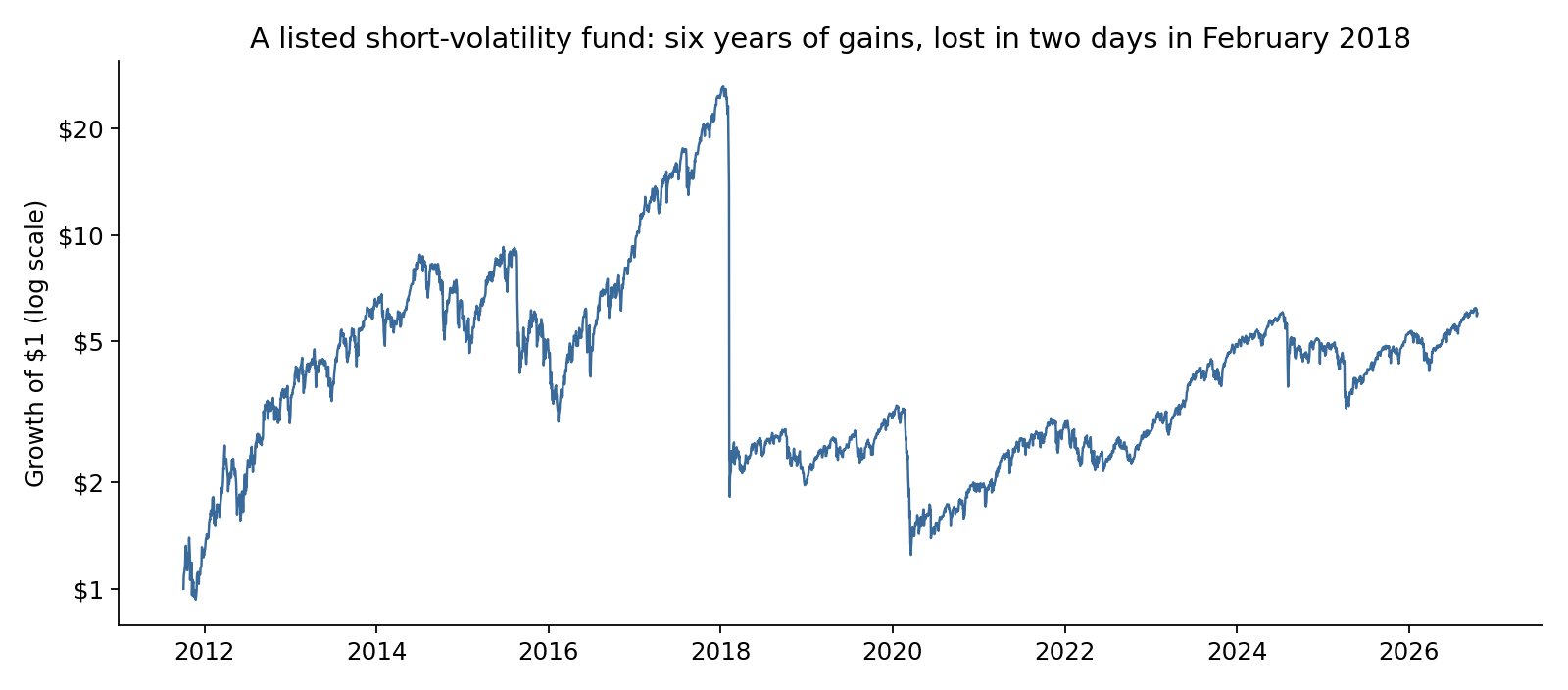
SVXY sold short-dated VIX futures every day. It earned the same premium, faster, and with daily rebalancing that turned a volatility spike into a near wipe-out in two sessions. The lesson is not that the premium disappeared; the fund has made money since. The lesson is that the structure and size of the position determined whether its holders survived the bad week.
Recommendations
- Decide the size from the tail, not the average. Set the vega notional so that the worst month on record costs a stated share of capital (5% of NAV in the illustration), and accept in writing a month twice as bad.
- Scale down as volatility rises. Size × 20 ÷ VIX doubled the premium per unit of tail risk in this sample and held in both halves. It is a rule, not a forecast.
- Fund the collateral before the trade. The loss arrives in days and margin calls arrive before the month ends. A short-volatility book needs liquid collateral sized to the stress month, held aside.
- Treat it as equity risk. Count the position against the equity risk budget and measure the whole portfolio in a crash month, when the short-volatility book and the equity book lose together.
- Monitor execution cost. At 1.5 vol points per trade the Sharpe ratio falls to 0.34; the premium is thin and must be bought and sold cheaply.
Limits
VIX approximates, but is not, a tradable variance-swap strike; real swaps trade at a spread to it and carry caps, margin and bid-ask that are covered only by the cost assumption. Realised volatility uses SPY closes rather than the index and closes rather than intraday paths. The sample has 365 monthly trades and its tail is defined by a handful of months, so the worst month on record is not the worst possible month. There is no model of mid-month margin calls or forced liquidation. This is independent research on public data; it is not investment advice and the strategy has not been deployed.

Sources
Data
- Cboe Volatility Index (VIX) daily history, Cboe Global Markets. Copy used: github.com/datasets/finance-vix (datahub core dataset, published under the PDDL)
- SPY and SVXY daily closes and SPY dividend events, Yahoo Finance. Copy used: huggingface.co/datasets/defeatbeta/yahoo-finance-data (ODC-BY)
Methods and documents referenced
- Cboe Global Markets. Cboe Volatility Index (VIX) White Paper.
- Demeterfi, K., Derman, E., Kamal, M. and Zou, J. (1999). "A Guide to Volatility and Variance Swaps." The Journal of Derivatives, 6(4), 9–32.
- Carr, P. and Wu, L. (2009). "Variance Risk Premiums." The Review of Financial Studies, 22(3), 1311–1341.
- ProShares Trust II, Form 8-K, Exhibit 99.1 (February 2018), on the change of SVXY's target exposure to -0.5x. sec.gov
Independent research, not investment advice. Dollar figures are illustrative. Analysis, code, charts and text were produced with AI assistance and reviewed by the author.