A ten-month moving-average rule is one of the best-known ideas in systematic investing: own equities while the market is above its ten-month average, hold Treasury bills when it is below. On 150 years of S&P 500 history it matches the market's return with far less risk, and cuts the Great Depression drawdown from -82% to -46%.
Tested on prices an investor could actually have traded at, about two-thirds of that advantage disappears. The rule still earns its place, but as crash insurance with a visible premium, not as a source of excess return. The difference matters for anyone sizing an overlay, setting a risk budget or reviewing a backtest.
Executive summary
The question. Should an equity allocation carry a trend-following overlay to limit crash losses, and what does that protection really cost?
The approach. Test two classic rules, the 10-month moving average and 12-month time-series momentum, on Robert Shiller's monthly S&P 500 data from 1871, then on SPY with dividends, real T-bill cash and trading costs from 1997. Run the identical rules on monthly-average and month-end SPY prices to isolate how the data is built. Every rule and cost was fixed before results were examined.
The answer. Long-history results are flattered by averaged prices, which leak part of the next month's move into the signal. On tradable prices the 10-month rule returned 9.2% a year against 9.8% for buy and hold, with a Sharpe ratio of 0.67 against 0.54, and cut the worst drawdown from -51% to -22%. It beat the market in only four of 28 calendar years.
The decision it supports. Treat trend following as a priced drawdown hedge, sized to the loss the portfolio cannot tolerate and judged against its insurance cost, and require tradable-price backtests for every systematic rule that reaches the investment committee.
Business outcomes
| Dimension | Buy and hold SPY | With the 10-month trend rule | What it means |
|---|---|---|---|
| Worst peak-to-trough loss | -51% (2007–09) | -22% | The tail is cut by more than half |
| Loss on a $1bn allocation at the worst point | About $508 million | About $218 million | About $290 million of capital preserved in the crisis |
| Annual return, 1997–2026 | 9.8% | 9.2% | The premium: about 0.6 points a year, roughly $6 million a year on $1bn |
| Annual return since June 2007 | 10.7% | 8.7% | In a long bull market the premium rises to about 2.0 points a year |
| Dot-com bust (Sep 2000–Oct 2002) | -40% | -5% | Slow, grinding bear markets are where the rule pays |
| Global financial crisis (Nov 2007–Mar 2009) | -47% | -3.5% | Same |
| COVID crash (Feb–Apr 2020) | -9% | -8% | Too fast for a monthly signal |
| Calendar years ahead / behind (28 full years) | n/a | Ahead in 4, behind in 17 | Expect to look wrong most years |
Tradable test: SPY month-end closes with dividends, cash in 3-month T-bills, 5 bp per switch. Dollar figures apply the measured percentages to an illustrative $1bn allocation. Episode returns are cumulative over the stated windows.
End to end in five steps
| Step | What happens | Output |
|---|---|---|
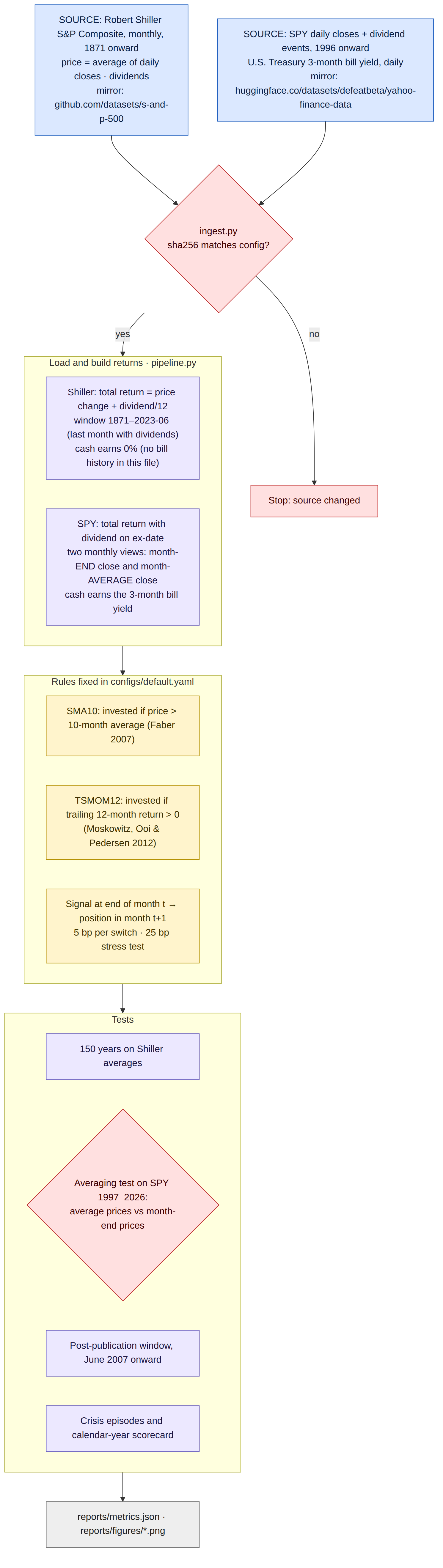
| 1. Source | Shiller monthly S&P 500 (1871 onward); SPY daily closes and dividends (1996 onward); 3-month T-bill yields; every file checksum-pinned | Raw data with provenance |
| 2. Build returns | Shiller total return from price plus dividend/12; SPY total return with ex-date dividends; month-end and month-average views of the same SPY history | Monthly return series |
| 3. Apply rules | 10-month moving average and 12-month momentum; signal at month-end t sets the position for month t+1 | Monthly positions |
| 4. Test | 150-year test, averaging test, post-publication window, crisis episodes, calendar-year scorecard, 25 bp cost stress | Performance and drawdown statistics |
| 5. Translate | Apply the measured drawdowns and return gaps to an illustrative $1bn allocation | Business outcomes table |
The data, and the problem hidden in it
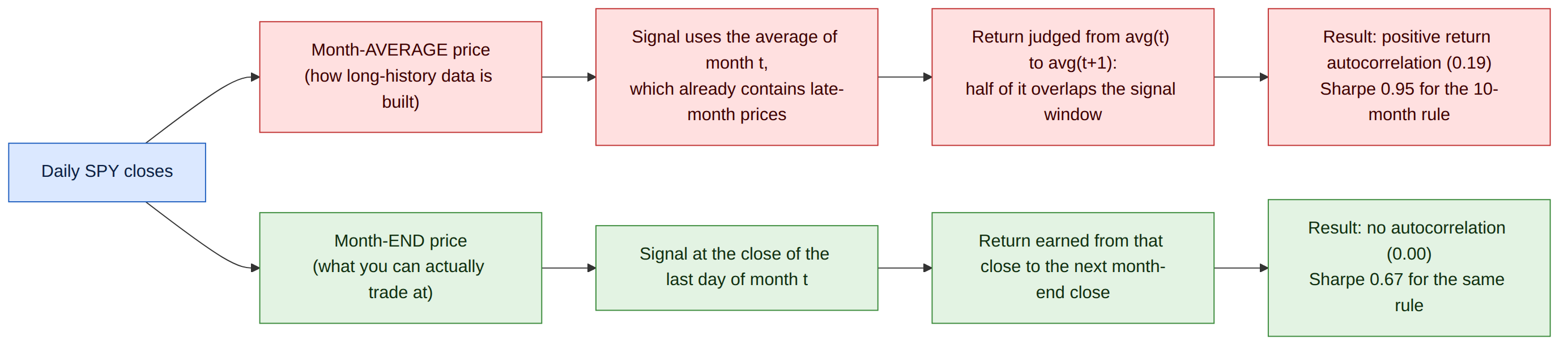
Robert Shiller's S&P 500 series is the backbone of much long-horizon research because it goes back to 1871 and includes dividends. Its monthly prices, however, are averages of daily closes across each month, not the price on the last trading day. That is a sensible choice for valuation work and a dangerous one for timing rules.
A signal built from a month's average already contains late-month prices. When that signal is judged on the return from one monthly average to the next, part of the move it is "predicting" has already happened. Holbrook Working showed in 1960 that averaging a random walk alone creates positive correlation between successive changes, and the data shows it plainly: lag-one autocorrelation of monthly returns is 0.27 in the Shiller series and 0.19 for averaged SPY prices, against 0.00 for SPY month-end prices. Trend rules are designed to harvest exactly that kind of persistence, so averaged data hands them an edge that cannot be traded.
The averaging test
To measure the effect directly, the identical rules were run on SPY over identical years, once with monthly-average prices and once with month-end prices.
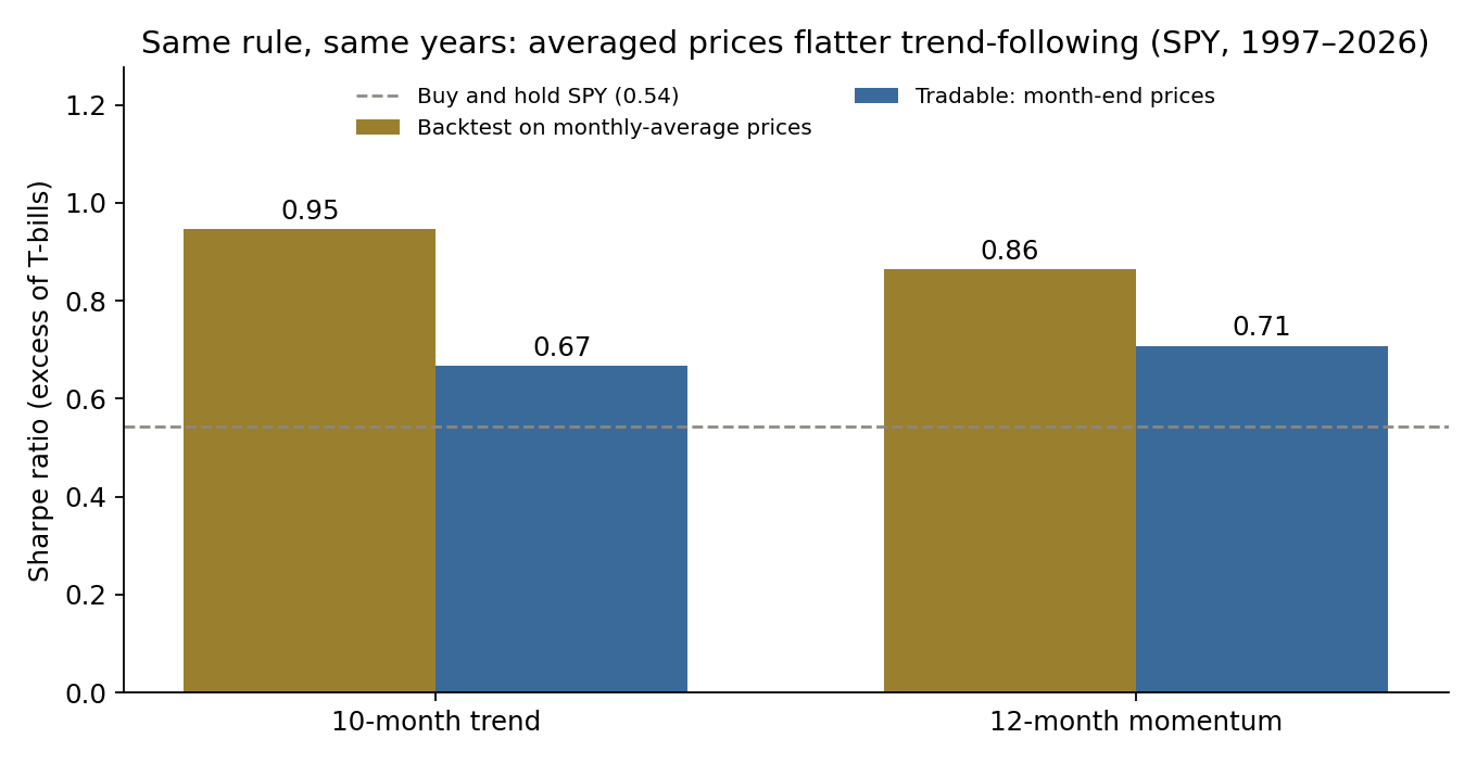
| SPY, 1997–2026 | Monthly-average prices | Month-end prices (tradable) |
|---|---|---|
| 10-month rule: annual return | 10.9% | 9.2% |
| 10-month rule: Sharpe ratio | 0.95 | 0.67 |
| 10-month rule: worst drawdown | -19% | -22% |
| 12-month momentum: Sharpe ratio | 0.86 | 0.71 |
| Buy and hold: Sharpe ratio | 0.62 | 0.54 |
| Lag-one autocorrelation of monthly returns | 0.19 | 0.00 |
Sharpe ratios in excess of 3-month T-bills. Buy and hold also looks smoother on averaged prices, which is why the comparison is made against each view's own buy-and-hold figure.
On averaged prices the 10-month rule improves the Sharpe ratio over buy and hold by 0.33. On tradable prices the improvement is 0.12. The 12-month momentum rule loses less of its edge, from 0.25 to 0.17, because its signal depends less on the last few weeks of prices.
The 150-year view, read correctly
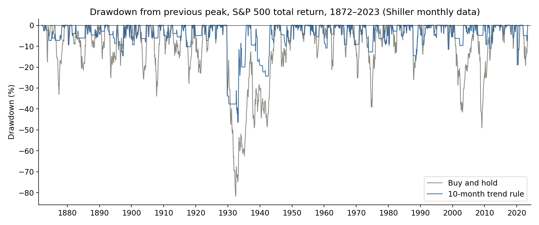
On the long history, the rule matched the market's return (9.2% against 9.1% a year), with a Sharpe ratio of 0.97 against 0.69 and a worst drawdown of -46% against -82%. Those figures appear in many presentations. They are directionally right: the rule has repeatedly stepped aside in long bear markets, including 1929–32. They are numerically optimistic for the reason above, so they should not be used to size a programme.
The tradable test
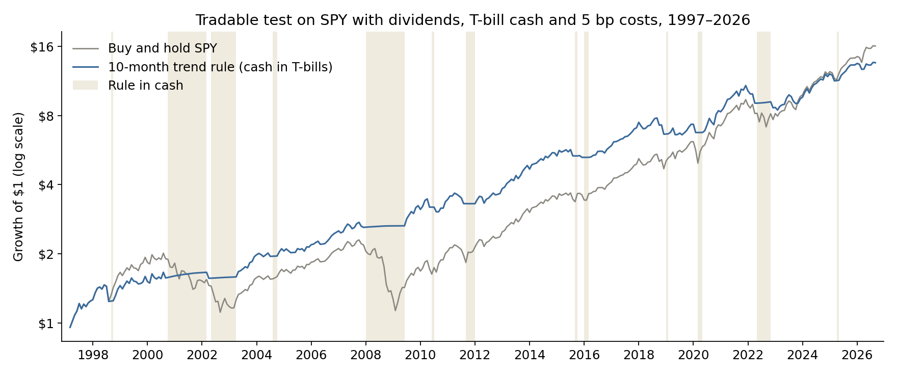
From 1997 to 2026 the 10-month rule returned 9.2% a year against 9.8% for buy and hold, with volatility of 10.7% against 15.3%, a Sharpe ratio of 0.67 against 0.54 and a worst drawdown of -22% against -51%. It held cash about a quarter of the time and switched about 1.5 times a year. A 25 bp cost per switch reduces the annual return by only 0.3 points, so trading cost is not the issue; timing is.
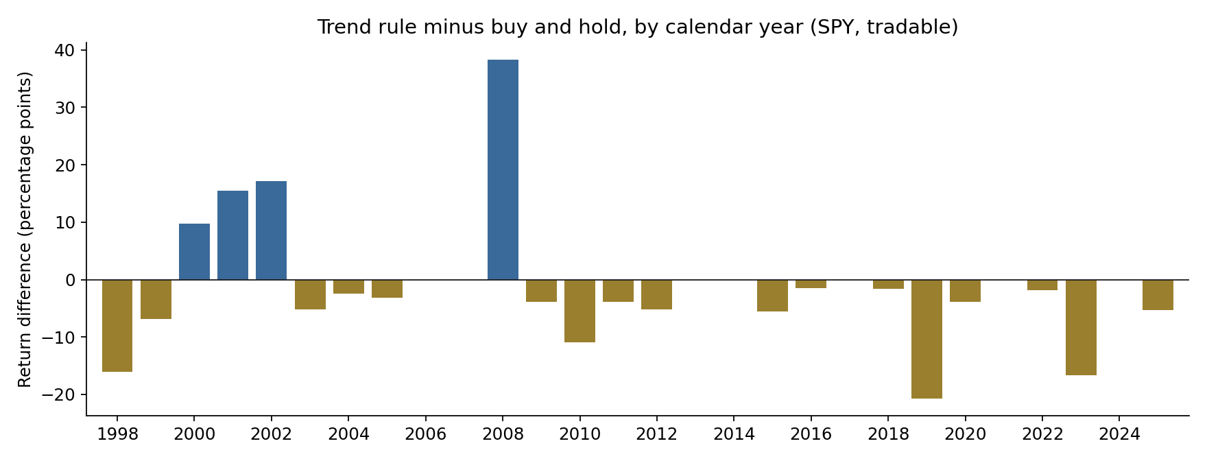
The scorecard is the most important exhibit for governance. In 28 full calendar years the rule was ahead by more than half a point in only four and behind in seventeen. It trailed by about 21 points in 2019 after selling in the late-2018 sell-off and buying back higher. It was too slow for the COVID crash and gave little protection in 2022. Its value is concentrated in a handful of slow, deep bear markets.
After the rule became well known
The 10-month rule was widely circulated from 2006–07. From June 2007, buy and hold returned 10.7% a year and the rule 8.7%; the worst drawdown fell from -51% to -22% and the Sharpe ratio was 0.70 against 0.64. The protection survived publication; the premium rose because the period was dominated by a long bull market.
Recommendations
- Classify trend overlays as hedges. Budget for them as insurance with an expected cost of roughly 0.5 to 2 points a year, not as return enhancers.
- Size to the binding constraint. The case is strongest where a deep drawdown would force selling, such as liquidity needs, leverage covenants or redemption risk. Without that constraint, the premium is harder to justify.
- Agree the losing years in advance. Expect to trail in most calendar years. Write the evaluation horizon and the switch-off criteria into the mandate before launch, so the overlay is not abandoned just before it is needed.
- Add a fast-crash complement. A monthly trend signal cannot react to a four-week crash. Pair it with volatility-based sizing or option protection if fast drawdowns are the concern.
- Make tradable-price backtests a standing control. Require every systematic rule to be tested on executable prices with costs, with the data construction disclosed, and report the averaging gap whenever long-history data is used.
Limits
This is a single asset. The long history uses averaged prices and zero cash return before 1990, so it is directional evidence only. Diversified trend programmes trade dozens of futures markets, with different costs and much better crisis records in some periods. SPY history covers about three decades and four major drawdowns. Nothing here is a forecast or investment advice.
Sources
Data
- Shiller, R. J. U.S. stock market data (S&P Composite price, dividends), from Irrational Exuberance and the accompanying online data, Yale University. Copy used: github.com/datasets/s-and-p-500
- SPY daily prices and dividend events, Yahoo Finance; U.S. Department of the Treasury daily par yield curve (3-month bill). Copy used: huggingface.co/datasets/defeatbeta/yahoo-finance-data (ODC-BY)
Methods referenced
- Faber, M. T. (2007). "A Quantitative Approach to Tactical Asset Allocation." The Journal of Wealth Management, 9(4), 69–79.
- Moskowitz, T. J., Ooi, Y. H. and Pedersen, L. H. (2012). "Time series momentum." Journal of Financial Economics, 104(2), 228–250.
- Working, H. (1960). "Note on the correlation of first differences of averages in a random chain." Econometrica, 28(4), 916–918.
Independent research, not investment advice. Dollar figures are illustrative. Analysis, code, charts and text were produced with AI assistance and reviewed by the author.